The Algorithm that Runs the World Can Now Run More of It
The most important algorithm, used for optimizing almost everything, is linear programming. New advances allow linear programming problems to be solved faster using the new commercial parallel simplex solver.
By Qi Huangfu, June 13, 2014.
“The algorithm that runs the world” said the cover story of a 2012 issue of the New Scientist Magazine. And yes, it was talking about the simplex algorithm. This topic is back in the news due to a major advance in the speed of the simplex algorithm as delivered by a commercial solution. The algorithm can now solve massive problems much more efficiently, frequently twice as fast as was previously possible.
Frankly, it is optimization that runs the world. By and large, running the modern world requires making many kinds of decisions: governments make decisions to allocate finite resources to advance society; companies make decisions to invest limited capital to generate more profit; and we all make personal decisions to spend our limited time on meaningful activities. This decision-making can take infinite forms. But to a mathematician, all decisions can be represented by mathematical models -- the allocation and limitation of the resources are regarded as variables and constraints, while the outcome is described by an objective function.
With this model ready, the next step is to solve it to optimality by identifying the decision that leads to the best possible outcome. The solution technique is called mathematical programming, or optimization. The simplex algorithm is at the very core of most optimization techniques. You could say the simplex algorithm runs the optimization world. It is either used to directly solve the relatively straightforward linear programming (LP) problems, or applied ubiquitously inside other more complicated optimization techniques.
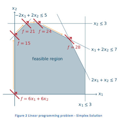
The simplex algorithm is an iterative algorithm for solving LP problems. The concept of LP can be illustrated by a small two-variable example in Figure 1. Here, we want to maximize a linear function (which could be the profit of investments) within the feasible region given by the linear constraints (which could be limitations of available resources). To solve such a simple example, one can draw its graphic representation and then easily use a pen or pencil to sweep through (pointing to the correct direction) the feasible region, until reaching the optimal extreme point. To solve the same problem using the simplex algorithm, the fundamental idea is still the same. The difference is that, rather than sweep through to the optimal point in a single shot, the simplex algorithm walks along the boundary of the feasible region, moving from one vertex to a more profitable one, until reaching the optimal vertex. Solving the same problem using the simplex algorithm is illustrated in Figure 2.
 Although it is convenient enough to solve trivial problems (up to 3 variables with a 3 dimensional graph) with pen or pencil, for anything larger than that, we need the simplex algorithm. As a matter of fact, nowadays, LP problems often consist of millions of variables that require an efficient simplex implementation.
While the theory behind the simplex algorithm is relatively simple, how to efficiently implement it in practice is more complex and has long been a major topic for research. Looking back at how the theory evolved since its introduction by George Dantzig in the 1940s, new ground-breaking research has been published roughly every decade, with the latest one being Hall and McKinnon’s hyper-sparsity algorithm in the first decade of the 21st Century. The simplex world has been relatively quiet since that publication, as if hyper-sparsity was the final brick to the well-polished simplex building.
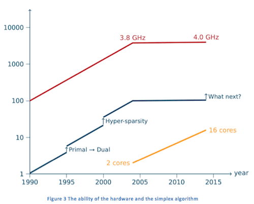
Besides the algorithmic improvement, advances in CPU performance have continuously boosted the power of the simplex algorithm. For example, a problem that took approximately 300 seconds to solve optimally in the 1970s can now be solved easily within 0.2 second -- some 1,500 times faster. A large fraction of the improvement came from the advance of CPU speed. However, “the free lunch is over”. The turning point was 2004, when the single-core speed of CPUs ceased to increase and mainstream manufacturers turned instead to increasing the number of cores in a CPU. This trend, together with the performance of the simplex solver, is plotted in Figure 3. In the graph, the red line illustrates the best-known single-core CPU clock frequency of mainstream manufacturers. From the 1990s to 2004, it increased some 40-fold from approximately 100 MHz to 3.8 GHz. We have seen hardly any increase since then, and only in June 2014 was Intel able to pass the 4 GHz barrier, a mere 5% improvement in 10 years. Note that it is not the CPU clock frequency alone that determines its performance, but it is widely accepted as a fair measure. On the other hand, as the yellow line shows, the number of cores in mainstream CPUs has shown a continuous growth in the last ten years as an alternative to further improve CPU performance.
What’s even more interesting is the performance of the simplex algorithm – by the standard measure of how many medium-sized LP problems can be solved in an hour – over this time period. The improvement has been a combination of the continuous CPU performance improvements and several leaps in ground-breaking algorithmic variants (linking the advances to the year the research was published). In the past, newer CPUs mean better performance. However, this stopped being true in 2004. Nowadays, the simplex solver needs to go parallel to still take advantage of the hardware evolution trend.
As a matter of fact, the simplex community has long tried parallelization, long before parallel computers were introduced to general daily usage. In the last 20 years, the many attempts have ranged from massively distributed machines in universities and national laboratories to modern GPUs in personal computers, using either dense or sparse matrix computations. However, good speed-up ratios always came from parallelizing less efficient sequential implementations of the simplex algorithm. As a result, the overall performance of these parallelization efforts is still inferior when compared to world-leading sequential simplex solvers.
A meaningful simplex parallelization has to be designed and developed based on a state-of-the-art sequential simplex solver and still allow for significant parallelization. This has been achieved in the most recent version of the FICO Xpress Optimization Suite. As the first commercial parallel simplex solver, it is able to solve various large-scale problems 2X faster (speedup of two) than other methods.
The key idea behind this implementation is to create more parallelizable scope by combining multiple simplex iterations into one “mega” simplex iteration. To implement this efficiently, several innovative techniques were developed. A detailed introduction to this approach is available here. The implementation in FICO Xpress is an adaption and further development of this key idea.
With this implementation, medium- to large-sized linear programming problems can often be solved 30% faster on average, in the best case up to 2 times faster. This introduced yet another performance leap to the simplex algorithm – while the search for other advances continues.
About the author

Qi Huangfu is the “simplex guy” behind the FICO Xpress Optimization Suite. Before joining FICO, he obtained a BSc in Computer Science from Beihang University in Beijing. He then earned an MSc in High Performance Computing and PhD in Mathematics from the University of Edinburgh. His PhD research topic was the parallel dual simplex method linked above. Notably, his PhD supervisor in Edinburgh, Julian Hall is the one who published the research on hyper-sparsity, resulting in the previous simplex performance leap.
Related:
“The algorithm that runs the world” said the cover story of a 2012 issue of the New Scientist Magazine. And yes, it was talking about the simplex algorithm. This topic is back in the news due to a major advance in the speed of the simplex algorithm as delivered by a commercial solution. The algorithm can now solve massive problems much more efficiently, frequently twice as fast as was previously possible.
Frankly, it is optimization that runs the world. By and large, running the modern world requires making many kinds of decisions: governments make decisions to allocate finite resources to advance society; companies make decisions to invest limited capital to generate more profit; and we all make personal decisions to spend our limited time on meaningful activities. This decision-making can take infinite forms. But to a mathematician, all decisions can be represented by mathematical models -- the allocation and limitation of the resources are regarded as variables and constraints, while the outcome is described by an objective function.
With this model ready, the next step is to solve it to optimality by identifying the decision that leads to the best possible outcome. The solution technique is called mathematical programming, or optimization. The simplex algorithm is at the very core of most optimization techniques. You could say the simplex algorithm runs the optimization world. It is either used to directly solve the relatively straightforward linear programming (LP) problems, or applied ubiquitously inside other more complicated optimization techniques.
The simplex algorithm is an iterative algorithm for solving LP problems. The concept of LP can be illustrated by a small two-variable example in Figure 1.
 Here, we want to maximize a linear function (which could be the profit of investments) within the feasible region given by the linear constraints (which could be limitations of available resources). To solve such a simple example, one can draw its graphic representation and then easily use a pen or pencil to sweep through (pointing to the correct direction) the feasible region, until reaching the optimal extreme point. To solve the same problem using the simplex algorithm, the fundamental idea is still the same. The difference is that, rather than sweep through to the optimal point in a single shot, the simplex algorithm walks along the boundary of the feasible region, moving from one vertex to a more profitable one, until reaching the optimal vertex. Solving the same problem using the simplex algorithm is illustrated in Figure 2.
 Although it is convenient enough to solve trivial problems (up to 3 variables with a 3 dimensional graph) with pen or pencil, for anything larger than that, we need the simplex algorithm. As a matter of fact, nowadays, LP problems often consist of millions of variables that require an efficient simplex implementation.
While the theory behind the simplex algorithm is relatively simple, how to efficiently implement it in practice is more complex and has long been a major topic for research. Looking back at how the theory evolved since its introduction by George Dantzig in the 1940s, new ground-breaking research has been published roughly every decade, with the latest one being Hall and McKinnon’s hyper-sparsity algorithm in the first decade of the 21st Century. The simplex world has been relatively quiet since that publication, as if hyper-sparsity was the final brick to the well-polished simplex building.
Besides the algorithmic improvement, advances in CPU performance have continuously boosted the power of the simplex algorithm. For example, a problem that took approximately 300 seconds to solve optimally in the 1970s can now be solved easily within 0.2 second -- some 1,500 times faster. A large fraction of the improvement came from the advance of CPU speed. However, “the free lunch is over”. The turning point was 2004, when the single-core speed of CPUs ceased to increase and mainstream manufacturers turned instead to increasing the number of cores in a CPU. This trend, together with the performance of the simplex solver, is plotted in Figure 3.
 In the graph, the red line illustrates the best-known single-core CPU clock frequency of mainstream manufacturers. From the 1990s to 2004, it increased some 40-fold from approximately 100 MHz to 3.8 GHz. We have seen hardly any increase since then, and only in June 2014 was Intel able to pass the 4 GHz barrier, a mere 5% improvement in 10 years. Note that it is not the CPU clock frequency alone that determines its performance, but it is widely accepted as a fair measure. On the other hand, as the yellow line shows, the number of cores in mainstream CPUs has shown a continuous growth in the last ten years as an alternative to further improve CPU performance.
What’s even more interesting is the performance of the simplex algorithm – by the standard measure of how many medium-sized LP problems can be solved in an hour – over this time period. The improvement has been a combination of the continuous CPU performance improvements and several leaps in ground-breaking algorithmic variants (linking the advances to the year the research was published). In the past, newer CPUs mean better performance. However, this stopped being true in 2004. Nowadays, the simplex solver needs to go parallel to still take advantage of the hardware evolution trend.
As a matter of fact, the simplex community has long tried parallelization, long before parallel computers were introduced to general daily usage. In the last 20 years, the many attempts have ranged from massively distributed machines in universities and national laboratories to modern GPUs in personal computers, using either dense or sparse matrix computations. However, good speed-up ratios always came from parallelizing less efficient sequential implementations of the simplex algorithm. As a result, the overall performance of these parallelization efforts is still inferior when compared to world-leading sequential simplex solvers.
A meaningful simplex parallelization has to be designed and developed based on a state-of-the-art sequential simplex solver and still allow for significant parallelization. This has been achieved in the most recent version of the FICO Xpress Optimization Suite. As the first commercial parallel simplex solver, it is able to solve various large-scale problems 2X faster (speedup of two) than other methods.
The key idea behind this implementation is to create more parallelizable scope by combining multiple simplex iterations into one “mega” simplex iteration. To implement this efficiently, several innovative techniques were developed. A detailed introduction to this approach is available here. The implementation in FICO Xpress is an adaption and further development of this key idea.
With this implementation, medium- to large-sized linear programming problems can often be solved 30% faster on average, in the best case up to 2 times faster. This introduced yet another performance leap to the simplex algorithm – while the search for other advances continues.
About the author

Qi Huangfu is the “simplex guy” behind the FICO Xpress Optimization Suite. Before joining FICO, he obtained a BSc in Computer Science from Beihang University in Beijing. He then earned an MSc in High Performance Computing and PhD in Mathematics from the University of Edinburgh. His PhD research topic was the parallel dual simplex method linked above. Notably, his PhD supervisor in Edinburgh, Julian Hall is the one who published the research on hyper-sparsity, resulting in the previous simplex performance leap.
Related:
- Are Big Data and Privacy at odds? FICO Interview
- How Deep Learning Analytics Mimic the Mind
- Evolution of Fraud Analytics – An Inside Story