Automotive Customer Churn Prediction Results, part 2
Learn how to apply neural networks and self-organizing maps to visualize the macroscopic relationships between clients and the maintenance evolution of cars over the years.
By Gregory Philippatos (www.directing.gr), Sep 2014
This is part 2 of the post - here is part 1.
Churn & Life Time Cycle
The need of a macroscopic point of view allowing us to see the relation between clients and maintenance evolution through years and the need to “visualize” this relation made us decided to use neural networks and self organizing map. As data and input variables we used the same as in the prediction model.
A self-organizing map consists of components called nodes or neurons. Associated with each node is a weight vector of the same dimension as the input data vectors and a position in the map space.
There is a visualization technique called the U-matrix or unified distance matrix that visualizes the distance between adjacent units in the SOM. It represents the map as a regular grid of neurons as illustrated in (Figure 2).

Based on features values of each cluster and on a clusters similitude’s analysis we observed that 4 Hyper Clusters are formed (Figure 3). Hyper Cluster A : clusters 4, 5, 10, 15, Hyper Cluster B : clusters 1, 2, 6, Hyper Cluster C : clusters 16, 17, 21, 22, Hyper Cluster D : clusters 19, 20, 23, 24, 25.

Based on real visits of cars who made maintenance service between 1/2/2014 and 31/7/2014 we observe that Hyper Cluster D is more important for car ages till 6 years, Hyper Cluster C for car ages between 6 and 10 and Hyper Cluster B for car ages over 10 years (Figure 5)


Related:
This is part 2 of the post - here is part 1.
Churn & Life Time Cycle
The need of a macroscopic point of view allowing us to see the relation between clients and maintenance evolution through years and the need to “visualize” this relation made us decided to use neural networks and self organizing map. As data and input variables we used the same as in the prediction model.
A self-organizing map consists of components called nodes or neurons. Associated with each node is a weight vector of the same dimension as the input data vectors and a position in the map space.
There is a visualization technique called the U-matrix or unified distance matrix that visualizes the distance between adjacent units in the SOM. It represents the map as a regular grid of neurons as illustrated in (Figure 2).
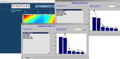
Figure 2. U-matrix visualization and clusters description
In order to interpret the map, and in particular the characteristics of each cluster, we used the component planes of the map that show the distribution of values across the map, according to one variable at a time (Figure 2)Based on features values of each cluster and on a clusters similitude’s analysis we observed that 4 Hyper Clusters are formed (Figure 3). Hyper Cluster A : clusters 4, 5, 10, 15, Hyper Cluster B : clusters 1, 2, 6, Hyper Cluster C : clusters 16, 17, 21, 22, Hyper Cluster D : clusters 19, 20, 23, 24, 25.
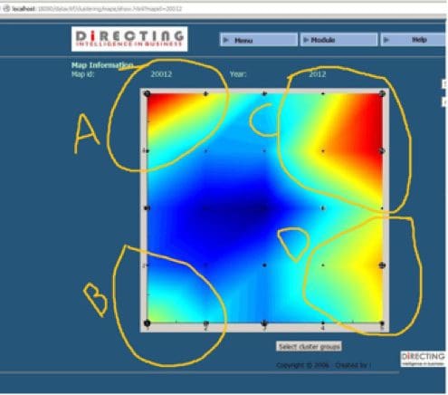
Figure 3. Hyper Clusters
Hyper Clusters and LTCBased on real visits of cars who made maintenance service between 1/2/2014 and 31/7/2014 we observe that Hyper Cluster D is more important for car ages till 6 years, Hyper Cluster C for car ages between 6 and 10 and Hyper Cluster B for car ages over 10 years (Figure 5)
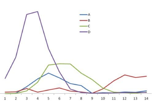
Figure 5. Relation between Hyper Clusters, real visits for maintenance and car age
Considering past years history we observe that from 2009 to 2014 there is a gradual movement from Hyper Cluster A to Hyper Clusters C and D, this movement allows us to predict that in 2015 we will have Hyper Cluster D as the only dominant. So Hyper Clusters allows us a macroscopic point of view of Life Time Cycle evolution through time (Figure 6)
Figure 6. Evolution of Hyper Clusters
Now concerning cars in warranty we observe a dominance of Hyper Cluster D independently of models (Figure 7) and for cars out of warranty we have a dominance of Hyper Cluster D for the Model_6 as it is the news of all and for the rest we have : Models 8, 1, 5, 4, 10 dominant Hyper Clusters are B and C, Models 2, 7 and 9, Hyper Clusters C and Model 3, Hyper Clusters B and D (Figure 8).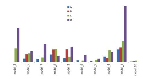
Figure 7. Cars < 6 years. Relation between Hyper Clusters, real visits and models
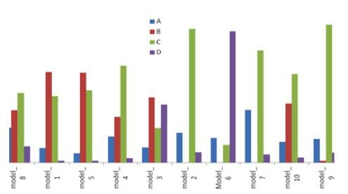
Figure 8. Cars > 6 years. Relation between Hyper Clusters, real visits and models
Gregory Philippatos is the principal at DIRECTING Intelligence in Business, based in Athens Greece, which creates Business Driven Analytics, applications of machine learning theory, tailored to specific industries and in each sector of industries to specific needs and business requirements of every company.Related: