Data Science of IoT: Sensor fusion and Kalman filters, Part 1

Introduction

This two part paper is created as part of the Data Science for IoT practitioners course(starting Nov 10) by Ajit Jaokar.  Kalman filters and sensor fusion is a hard topic and has implications for IoT.  I  welcome comments and feedback at ajit.jaokar at futuretext.com. Please email us at info at futuretext.com if you want to join the Data Science for IoT practitioners course.

Kalman filtering is an algorithm that uses a series of measurements observed over time, containing statistical noise and other inaccuracies, and produces estimates of unknown variables that tend to be more precise than those based on a single measurement alone (adapted from Wikipedia).  The Kalman filter has numerous applications in technology – including IoT.  Specifically, Kalman filters are used in Sensor fusion. Sensor fusion helps to determine the State (and also the overall Context) of an IoT based computing system which relies on inferring the combined meaning from different sensors.

In Part One, we describe the workings of Kalman filters and in Part Two we describe the implications for IoT devices.

Examples of usage

Kalman filters are best introduced through examples:

Prediction of water level: Suppose you have a  model that predicts river water level every hour (using the usual inputs).  You know that your model is not perfect and you don’t trust it 100%. So you want to send someone to check the river level in person. However, the river level can only be checked once a day around noon and not every hour. Furthermore, the person who measures the river level cannot be trusted 100% either. So how do you combine both outputs of river level (from model and from measurement) so that you get a ‘fused’ and better estimate?  Source: Introduction to Kalman filters – CEE 6430: Probabilistic Methods in Hydrosciences – Fall 2008

Determining location of a Truck: Consider the problem of determining the precise location of a truck. The truck can be equipped with a GPS unit that provides an estimate of the position within a few meters. The GPS estimate is likely to be noisy; readings ‘jump around’ rapidly, though always remaining within a few meters of the real position. In addition, since the truck is expected to follow the laws of physics, its position can also be estimated by integrating its velocity over time, determined by keeping track of wheel revolutions and the angle of the steering wheel. This is a technique known as dead reckoning. Typically, dead reckoning will provide a very smooth estimate of the truck’s position, but it will drift over time as small errors accumulate.

In this example, the Kalman filter can be thought of as operating in two distinct phases: predict and update. In the prediction phase, the truck’s old position will be modified according to the physical laws of motion (the dynamic or “state transition” model) plus any changes produced by the accelerator pedal and steering wheel. We also update the covariance between the two variables.

In probability theory and statistics, covariance is a measure of how much two random variables change together. If the greater values of one variable mainly correspond with the greater values of the other variable, and the same holds for the smaller values, i.e., the variables tend to show similar behaviour, the covariance is positive. In the opposite case, when the greater values of one variable mainly correspond to the smaller values of the other, i.e., the variables tend to show opposite behaviour, the covariance is negative. The sign of the covariance therefore shows the tendency in the linear relationship between the variables.

Not only will a new position estimate be calculated, but a new covariance will be calculated as well. The covariance is proportional to the ‘greater certainity’ metric (perhaps speed of the truck). Subsequent updates will create more accurate readings.

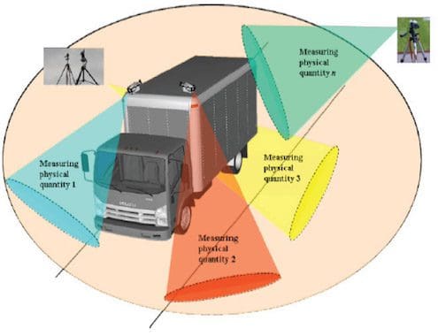
Image: http://spie.org/x108745.xml depicting multisensory surveillance for a moving vehicle. Note that it is different application of Kalman filters from the one discussed above – but the same principles apply. Example of Truck positioning – adapted from wikipedia

Initial concepts

Here are some initial points:

• The system state cannot be measured directly
• There are multiple measurements – each of which are not accurate/ These need to be fused/combined.
• Fusion across different Sensors can mean different things: Example: several temperature sensors, Fusion across different Attributes, (Example: Temperature, pressure humidity to determine air refractive index), Fusion across different Domains, Example: different ranges / domains, Fusion across different Time (Example: Sampling over space and time) [adapted Boujemaa and Forbes, 2007]
• Note, Sensor fusion is not merely ‘adding’ values i.e. not just adding temperatures. It is more about understanding the overall ‘State’ of a system based on multiple sensors. (see below for meaning of State in this context)

In the next part of this post, we explore the workings of Kalman filters and their impact on sensor fusion on IoT.

This two part paper is created as part of the Data Science for IoT practitioners course(starting Nov 10) by Ajit Jaokar.  Please email us at info at futuretext.com if you want to join the Data Science for IoT practitioners course.

Many thanks to Dr Gary Butler – founder and CEO of Camgian Microsystems and Karthik Padbanabhan – manager Smart mobility at Ford Motor Company for their comments.

Related:

• How Big Data Helps Build Smart Cities
• Impact of IoT on Big Data Landscape
• Data Science for Internet of Things – practitioner course