Tree Kernels: Quantifying Similarity Among Tree-Structured Data

Kernel Methods

Kernel methods avoid the need to convert data into vector form. The only information they require is a measurement of the similarity of each pair of items in a data set. This measurement is called a kernel, and the function for determining it is called the kernel function. Kernel methods look for linear relations in the feature space. Functionally, they are equivalent to taking the dot product of two data points in the feature space, and indeed feature design may still be a useful step in kernel function design. However, kernel methods methods avoid directly operating on the feature space since it can be shown that it’s possible to replace the dot product with a kernel function, as long as the kernel function is a symmetric, positive semidefinite function which can take as inputs the data in its original space.

The advantage of using kernel functions is thus that a huge feature space can be analyzed with a computational complexity not dependent on the size of the feature space, but on the complexity of the kernel function, which means that kernel methods do not to suffer the curse of dimensionality.

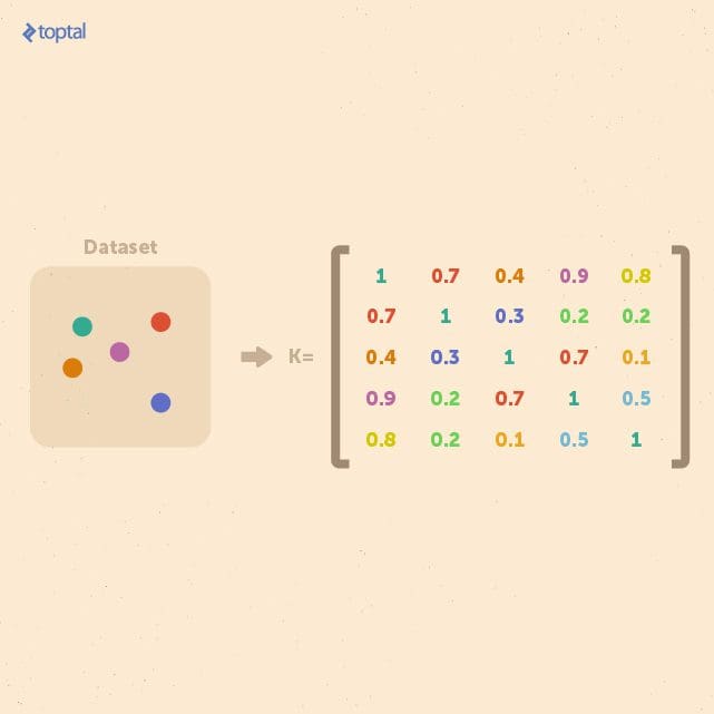
If we consider a finite dataset composed of n examples, we can get a complete representation of similarities within the data by generating a kernel matrix whose size is always n × n. This matrix is independent of the size of each individual example. This property is useful when a small dataset of examples with a large feature space is to be analyzed.

In general, kernel methods are based on a different answer to the question of data representation. Instead of mapping the input points into a feature space, the data is represented via pairwise comparisons in a kernel matrix K, and all relevant analysis can be performed over the kernel matrix.

Many data mining methods can be kernelized. To classify tree-structured data instances with kernel methods, such as with support vector machines, it suffices to define a valid (symmetric positive definite) kernel function k : T × T → R, also referred to as a tree kernel. In the design of practically useful tree kernels, one would require them to be computable in polynomial time over the size of the tree, and to be able to detect isomorphic graphs. Such tree kernels are called complete tree kernels.

Tree Kernels

Now, let’s introduce some useful tree kernels for measuring the similarity of trees. The main idea is to calculate the kernel for each pair of trees in the data set in order to build a kernel matrix, which can then be used for classifying sets of trees.

String Kernel

First, we will start with a short introduction to string kernels, which will help us to introduce another kernel method that is based on converting trees into strings.

Let’s define num_y(s) as the number of occurrences of a substring y in a string s, with |s| denoting the length of string. The string kernel that we shall describe here is defined as:

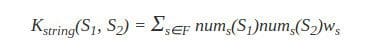
Where F is the set of substrings that occur in both S₁ and S₂, and the parameter w_s serves as a weight parameter (for example, to emphasize important substrings). As we can see, this kernel gives a higher value to a pair of strings when they share many common substrings.

Tree Kernel Based on Converting Trees into Strings

We can use this string kernel to build a tree kernel. The idea behind this kernel is to convert two trees into two strings in a systematic way that encodes the tree’s structure, and then apply the above string kernel to them.

We convert the two trees into two strings as follows:

Let T denote one of the target trees, and label(n_s) the string label of node n_s in T. tag(n_s) denotes the string representation of the subtree of T rooted at n_s. So if n_root is the root node of T, tag(n_root) is the string representation of the entire tree T.

Next, let string(T) = tag(n_root) denote the string representation of T. We will recursively apply the following steps in a bottom-up fashion to obtain string(T):

• If the node n_s is a leaf, let tag(n_s) = “[” + label(n_s) + “]” (where + here is the string concatenation operator).
• If the node _ns is not a leaf and has c children n₁, n₂, … , n_c, sort tag(n₁), tag(n₂), … , tag(n_c) in lexical order to obtain tag(n_1*), tag(n_2*), … , tag(n_c*), and let tag(n_s) = “[” + label(n_s) + tag(n_1*) + tag(n_2*) + … + tag(n_c*) + “]”.

The figure below, shows an example of this tree-to-string conversion. The result is a string starting with an opening delimiter such as “[” and ending with its closing counterpart, “]”, with each nested pair of delimiters corresponding to a subtree rooted at a particular node.

Now we can apply the above conversion to two trees, T₁ and T₂, to obtain two strings S₁ and S₂. From there, we can simply apply the string kernel described above.

The tree kernel between T₁ and T₂ via two strings S₁ and S₂ can now be given as:

In most applications, the weight parameter becomes w_|s|, weighting a substring based on its length |s|. Typical weighting methods for w_|s| are:

• constant weighting (w_|s| = 1)
• k-spectrum weighting (w_|s| = 1 if |s| = k, and w_|s| = 0 otherwise)
• exponential weighting (w_|s| = λ_|s| where 0 ≤ λ ≤ 1 is a decaying rate)

To compute the kernel, it’s sufficient to determine all of the common substrings F, and to count the number of times they occur in S₁ and S₂. This additional step of finding common substrings is a well-studied problem, and can be accomplished in O(|S₁| + |S₂|), employing suffix trees or suffix arrays. If we assume that the maximum number of letters (bits, bytes, or characters, for example) needed to describe a node’s label is constant, the lengths of the converted strings are |S₁| = O(|T₁|) and |S₂| = O(|T₂|). So, the computational complexity of computing the kernel function is O(|T₁| + |T₂|), which is linear.