9 Key Deep Learning Papers, Explained

6. Region Based CNNs (R-CNN - 2013, Fast R-CNN - 2015, Faster R-CNN - 2015)

 
Some may argue that the advent of R-CNNs has been more impactful that any of the previous papers on new network architectures. With the first R-CNN paper being cited over 1600 times, Ross Girshick and his group at UC Berkeley created one of the most impactful advancements in computer vision. As evident by their titles, Fast R-CNN and Faster R-CNN worked to make the model faster and better suited for modern object detection tasks.

The purpose of R-CNNs is to solve the problem of object detection. Given a certain image, we want to be able to draw bounding boxes over all of the objects. The process can be split into two general components, the region proposal step and the classification step.

The authors note that any class agnostic region proposal method should fit. Selective Search is used in particular for RCNN. Selective Search performs the function of generating 2000 different regions that have the highest probability of containing an object. After we’ve come up with a set of region proposals, these proposals are then “warped” into an image size that can be fed into a trained CNN (AlexNet in this case) that extracts a feature vector for each region. This vector is then used as the input to a set of linear SVMs that are trained for each class and output a classification. The vector also gets fed into a bounding box regressor to obtain the most accurate coordinates.

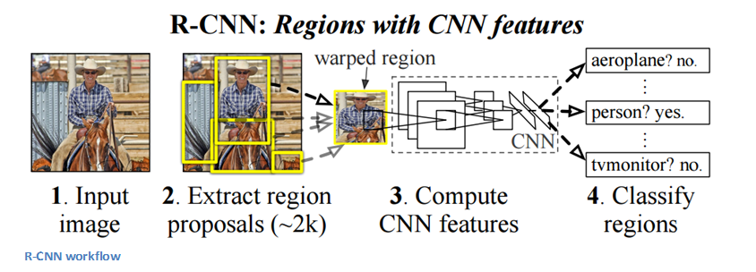
Non-maxima suppression is then used to suppress bounding boxes that have a significant overlap with each other.

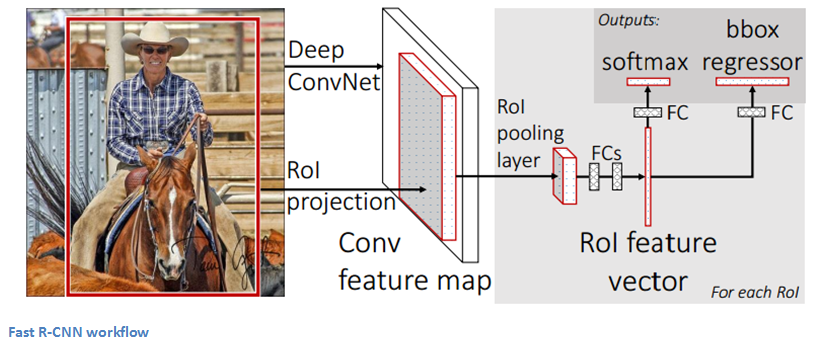
Fast R-CNN

Improvements were made to the original model because of 3 main problems. Training took multiple stages (ConvNets to SVMs to bounding box regressors), was computationally expensive, and was extremely slow (RCNN took 53 seconds per image). Fast R-CNN was able to solve the problem of speed by basically sharing computation of the conv layers between different proposals and swapping the order of generating region proposals and running the CNN. In this model, the image is firstfed through a ConvNet, features of the region proposals are obtained from the last feature map of the ConvNet (check section 2.1 of the paper for more details), and lastly we have our fully connected layers as well as our regression and classification heads.

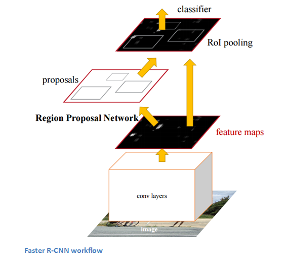
Faster R-CNN

Faster R-CNN works to combat the somewhat complex training pipeline that both R-CNN and Fast R-CNN exhibited. The authors insert a region proposal network (RPN) after the last convolutional layer. This network is able to just look at the last convolutional feature map and produce region proposals from that. From that stage, the same pipeline as R-CNN is used (ROI pooling, FC, and then classification and regression heads).

Why It’s Important

Being able to determine that a specific object is in an image is one thing, but being able to determine that object’s exact location is a huge jump in knowledge for the computer. Faster R-CNN has become the standard for object detection programs today.

7. Generative Adversarial Networks (2014)

 
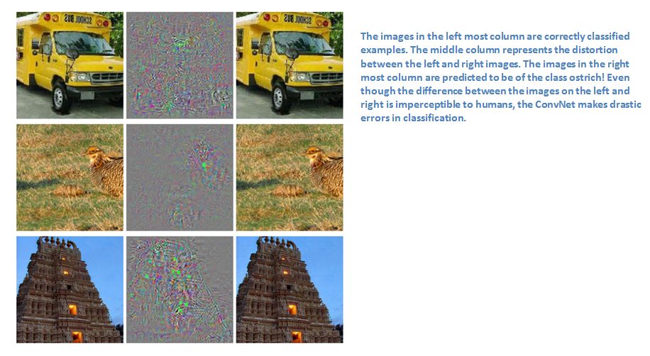
According to Yann LeCun, these networks could be the next big development. Before talking about this paper, let’s talk a little about adversarial examples. For example, let’s consider a trained CNN that works well on ImageNet data. Let’s take an example image and apply a perturbation, or a slight modification, so that the prediction error is maximized. Thus, the object category of the prediction changes, while the image itself looks the same when compared to the image without the perturbation. From the highest level, adversarial examples are basically the images that fool ConvNets.

Adversarial examples (paper) definitely surprised a lot of researchers and quickly became a topic of interest. Now let’s talk about the generative adversarial networks. Let’s think of two models, a generative model and a discriminative model. The discriminative model has the task of determining whether a given image looks natural (an image from the dataset) or looks like it has been artificially created. The task of the generator is to create images so that the discriminator gets trained to produce the correct outputs. This can be thought of as a zero-sum or minimax two player game. The analogy used in the paper is that the generative model is like “a team of counterfeiters, trying to produce and use fake currency” while the discriminative model is like “the police, trying to detect the counterfeit currency”. The generator is trying to fool the discriminator while the discriminator is trying to not get fooled by the generator. As the models train, both methods are improved until a point where the “counterfeits are indistinguishable from the genuine articles”.

Why It’s Important

Sounds simple enough, but why do we care about these networks? As Yann LeCun stated in his Quora post, the discriminator now is aware of the “internal representation of the data” because it has been trained to understand the differences between real images from the dataset and artificially created ones. Thus, it can be used as a feature extractor that you can use in a CNN. Plus, you can just create really cool artificial images that look pretty natural to me (link).

8. Generating Image Descriptions (2014)

 
What happens when you combine CNNs with RNNs (No, you don’t get R-CNNs, sorry )?But you do get one really amazing application. Written by Andrej Karpathy (one of my personal favorite authors) and Fei-Fei Li, this paper looks into a combination of CNNs and bidirectional RNNs (Recurrent Neural Networks) to generate natural language descriptions of different image regions. Basically, the model is able to take in an image, and output this:

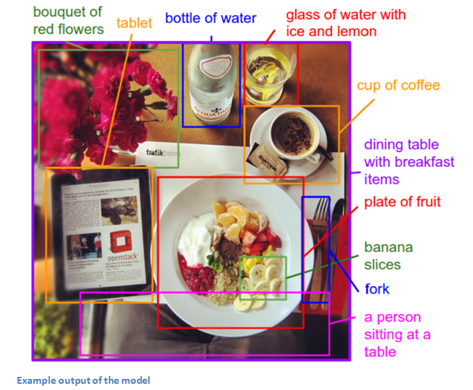
That’s pretty incredible. Let’s look at how this compares to normal CNNs. With traditional CNNs, there is a single clear label associated with each image in the training data. The model described in the paper has training examples that have a sentence (or caption) associated with each image. This type of label is called a weak label, where segments of the sentence refer to (unknown) parts of the image. Using this training data, a deep neural network “infers the latent alignment between segments of the sentences and the region that they describe” (quote from the paper). Another neural net takes in the image as input and generates a description in text. Let’s take a separate look at the two components, alignment and generation.

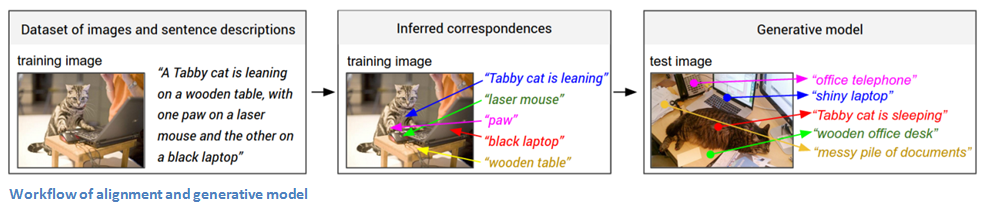
Alignment Model

The goal of this part of the model is to be able to align the visual and textual data (the image and its sentence description). The model works by accepting an image and a sentence as input, where the output is a score for how well they match (Now, Karpathy refers a different paper which goes into the specifics of how this works. This model is trained on compatible and incompatible image-sentence pairs).

Now let’s think about representing the images. The first step is feeding the image into an R-CNN in order to detect the individual objects. This R-CNN was trained on ImageNet data. The top 19 (plus the original image) object regions are embedded to a 500 dimensional space. Now we have 20 different 500 dimensional vectors (represented by v in the paper) for each image. We have information about the image. Now, we want information about the sentence. We’re going to embed words into this same multimodal space. This is done by using a bidirectional recurrent neural network. From the highest level, this serves to illustrate information about the context of words in a given sentence. Since this information about the picture and the sentence are both in the same space, we can compute inner products to show a measure of similarity.

Generation Model

The alignment model has the main purpose of creating a dataset where you have a set of image regions (found by the RCNN) and corresponding text (thanks to the BRNN). Now, the generation model is going to learn from that dataset in order to generate descriptions given an image. The model takes in an image and feeds it through a CNN. The softmax layer is disregarded as the outputs of the fully connected layer become the inputs to another RNN. For those that aren’t as familiar with RNNs, their function is to basically form probability distributions on the different words in a sentence (RNNs also need to be trained just like CNNs do).

Disclaimer: This was definitely one of the more dense papers in this section, so if anyone has any corrections or other explanations, I’d love to hear them in the comments!

Why It’s Important

The interesting idea for me was that of using these seemingly different RNN and CNN models to create a very useful application that in a way combines the fields of Computer Vision and Natural Language Processing. It opens the door for new ideas in terms of how to make computers and models smarter when dealing with tasks that cross different fields.

9. Spatial Transformer Networks (2015)

 
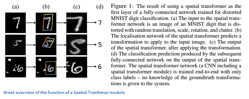
Last, but not least, let’s get into one of the more recent papers in the field. This paper was written by a group at Google Deepmind a little over a year ago. The main contribution is the introduction of a Spatial Transformer module. The basic idea is that this module transforms the input image in a way so that the subsequent layers have an easier time making a classification. Instead of making changes to the main CNN architecture itself, the authors worry about making changes to the image before it is fed into the specific conv layer. The 2 things that this module hopes to correct are pose normalization (scenarios where the object is tilted or scaled) and spatial attention (bringing attention to the correct object in a crowded image). For traditional CNNs, if you wanted to make your model invariant to images with different scales and rotations, you’d need a lot of training examples for the model to learn properly. Let’s get into the specifics of how this transformer module helps combat that problem.

The entity in traditional CNN models that dealt with spatial invariance was the maxpooling layer. The intuitive reasoning behind this later was that once we know that a specific feature is in the original input volume (wherever there are high activation values), it’s exact location is not as important as its relative location to other features. This new spatial transformer is dynamic in a way that it will produce different behavior (different distortions/transformations) for each input image. It’s not just as simple and pre-defined as a traditional maxpool. Let’s take look at how this transformer module works. The module consists of:

• A localization network which takes in the input volume and outputs parameters of the spatial transformation that should be applied. The parameters, or theta, can be 6 dimensional for an affine transformation.
• The creation of a sampling grid that is the result of warping the regular grid with the affine transformation (theta) created in the localization network.
• A sampler whose purpose is to perform a warping of the input feature map.

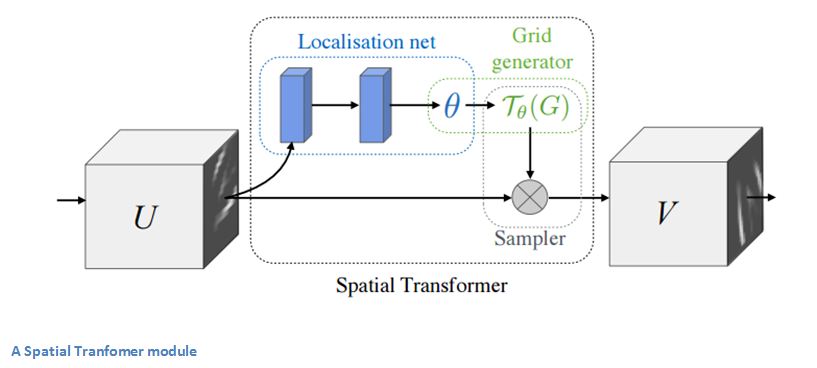
This module can be dropped into a CNN at any point and basically helps the network learn how to transform feature maps in a way that minimizes the cost function during training.

Why It’s Important

This paper caught my eye for the main reason that improvements in CNNs don’t necessarily have to come from drastic changes in network architecture. We don’t need to create the next ResNet or Inception module. This paper implements the simple idea of making affine transformations to the input image in order to help models become more invariant to translation, scale, and rotation. For those interested, here is a video from Deepmind that has a great animation of the results of placing a Spatial Transformer module in a CNN and a good Quora discussion.

And that ends our 3 part series on ConvNets! Hope everyone was able to follow along, and if you feel that I may have left something important out, let me know in the comments! If you want more info on some of these concepts, I once again highly recommend Stanford CS 231n lecture videos which can be found with a simple YouTube search.

Bio: Adit Deshpande is currently a second year undergraduate student majoring in computer science and minoring in Bioinformatics at UCLA. He is passionate about applying his knowledge of machine learning and computer vision to areas in healthcare where better solutions can be engineered for doctors and patients.

Original. Reposted with permission.

Related:

• A Beginner’s Guide To Understanding Convolutional Neural Networks Part 1
• Deep Learning in Neural Networks: An Overview
• 3 Thoughts on Why Deep Learning Works So Well