Deep Learning Research Review: Reinforcement Learning

DQN For Reinforcement Learning (RL With Atari Games)

 

Introduction

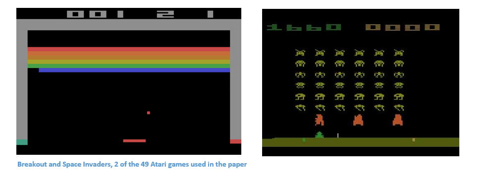
This paper was published by Google Deepmind in February of 2015 and graced the cover of Nature, a world famous weekly journal of science. This was one of the first successful attempts at combining deep neural networks with reinforcement learning (This was Deepmind’s original paper). The paper showed that their system was able to play Atari games at a level comparable to professional game testers across a set of 49 games. Let’s take a look at how they did it.

Approach

Okay, so remember where we left off in the intro tutorial at the beginning of the post? We had just described the main goal of having to optimize our action value function Q. The folks at Deepmind approached this task through a Deep Q-Network, or a DQN. This network is able to come up with successful policies that optimize Q, all from inputs in the form of pixels from the game screen and the current score.

Network Architecture

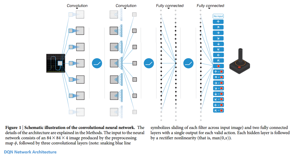
Let’s take a closer look at what inputs this DQN will have. Consider the game of Breakout, and take 4 of the most recent frames in the current game. Each of these frame originally starts as a 210 x 160 x 3 image (because width and height are 210 and 160 pixels and it is a color image). Then, some preprocessing takes place where the frames are scaled to 84 x 84 (not extremely important to know how this is done, but check page 6 for details). So, now we have an 84 x 84 x 4 input volume.  This volume is going to get plugged into a convolutional neural network (tutorial) where it will go through a series of conv and ReLU layers. The output of the network is an 18 dimensional vector where each number is the Q-value for each possible action the user can take (move up, down, left, etc).

Okay, so let’s take a step back for a second and figure out how we’re going to train this network so that It will predict accurate Q-values. Let’s first remember what we’re trying to optimize.

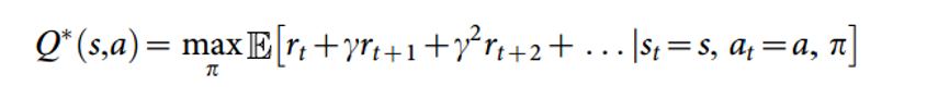
This is the same form as the Q function we saw earlier, except this one represents Q* which is the max over all Q’s. Let’s examine how we’re going to get this Q*. Now, remember we just want an approximation for Q*, which is where our function approximators are going to come in (our Qhats). Just keep that thought in your head while we switch gears a little.

In order to find the best policy, we want to frame some sort of supervised learning problem where the predicted Q function is compared to some expected one, and then is adjusted in the correct direction. In order to do that, we need a set of training examples. In our case, we are going to have to create a set of experiences that store the agent’s state, action, reward, and next state for every time step. Let’s formalize that a bit more. We have a replay memory D which contains (st, at, rt, st+1) for a bunch of different time steps. This dataset gets built over time, as the agent interacts more with the environment. Now, we’re going a take a random batch of this data (let’s say data for 64 time steps), compute the loss function for each of them, and then follow the gradient to improve our Q function approximation.

So, as you can see, the loss function wants to optimize the mean squared error (MSE) between the Q network function approximation (Q(s,a,theta)) and the Q learning targets. Let me quickly explain those.  This Q learning target is the reward r plus the maximum Q value (in the next time step) that you can get from some action a’.

Once the loss function is computed, the derivatives are taken w.r.t the theta values (or the w vector). These values are then updated so as to minimize the loss function.

Conclusion

One of my favorite parts about the paper is this visualization it gives of the value function during certain points of the game.

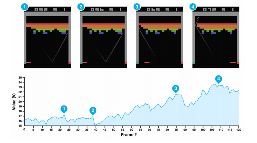
As you remember, the value function is basically a metric for measuring “how good it is to be in a particular situation”. If you look at #4, you can see, based on the trajectory of the ball and the location of the bricks, that we’re in for a lot of points and the high value function is quite representative of that.

All 49 Atari games used the same network architecture, algorithm, and hyperparameters which is an impressive testament to the robustness of such an approach to reinforcement learning. The combination of deep networks and traditional reinforcement learning strategies, like Q learning, proved to be a great breakthrough in setting the stage for...

Mastering AlphaGo with RL

 

Introduction

4-1. That’s the record Deepmind’s RL agent had against one of the best Go players in the world, Lee Sedol. In case you didn’t know, Go is an abstract strategy game of capturing territory on a game board. It is considered to be one of the hardest games in the world for AI because of the incredible number of different game scenarios and moves. The paper begins with a comparison of Go and common board games like chess and checkers. While those can be attacked with variations of tree search algorithms, Go is a totally different animal because there are about 250150 different sequences of moves in a game. It’s clear that reinforcement learning was needed, so let’s look into how AlphaGo managed to beat the odds.

Approach

The basis behind AlphaGo are the ideas of evaluation and selection. With any reinforcement learning problem (especially with a board game), you need a way of evaluating the environment, or the current board position. This is going to be our value network. You then need a way of selecting an action to take through a policy network. We’ve definitely had experience with both of these terms, value and policy.

Network Architecture

Let’s look at what inputs both of these networks are going to take. The board position is passed in as a 19 x 19 image that goes through a series of conv layers to construct a good representation of the current state. So let’s first look at our SL (Supervised Learning) policy network. This network is going to take in the image as input and then output a probability distribution over all of the legal actions the agent can take. This network is pretrained (before the actual game) on 30 million different Go board positions. Each of these board positions is labeled with what an expert move would be in that situation. The team also trained a smaller, but faster rollout policy network.

Now, CNNs can only do so much to predict the correct move you should take, given a representation of the current board. That’s when reinforcement learning comes in. We’re going to improve this policy network through a process called policy gradients. Remember how in the last paper, we wanted to optimize our action value function Q? Well now, we’re going straight to optimizing our policy (Policy gradients take a while to explain but David Silver does a good job in Lecture 7). From a high level, the policy is improved by simulating games between the current policy network and a previous iteration of the network. The reward signal is +1 for winning the game, -1 for losing, and so we can improve the network through the normal gradient descent.

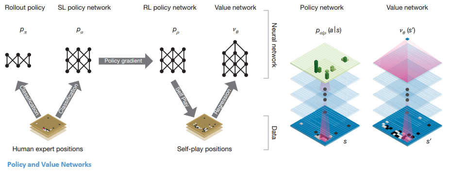
Okay, so now we have a pretty good network that tells us the best action to play. The next step is having a value network that predicts the outcome a game which is at board position S and where both players are using policy P.

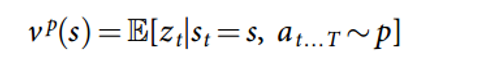
In order to get the optimal V*, we’ll use our good old function approximators with weights W. The weights are trained by the value network which are conditioned on state, outcome pairs (similar to what we saw in the last paper).

Now that we have these main two networks, our final step is to use a Monte Carlo Tree Search to put everything together. The basic idea behind MCTS is that it selects the best actions through lookahead search where each edge in the tree stores an action value Q, a visit count, and a prior probability. From that info, the MCTS algorithm will pick the best action A from the current state. This part of the system is a little less RL and more traditional AI so if you’d like more details, definitely check out the paper, which will do a much better job of summarizing.

Conclusion

A computer system just beat the world’s best player at one of the hardest board games ever. Who even needs a conclusion?

via GIPHY

Big thanks to David Silver for the equations and the excellent lecture course on RL

Bio: Adit Deshpande is currently a second year undergraduate student majoring in computer science and minoring in Bioinformatics at UCLA. He is passionate about applying his knowledge of machine learning and computer vision to areas in healthcare where better solutions can be engineered for doctors and patients.

Original. Reposted with permission.

Related:

• Deep Learning Research Review: Generative Adversarial Nets
• Deep Learning in Neural Networks: An Overview
• 9 Key Deep Learning Papers, Explained