An Intuitive Explanation of Convolutional Neural Networks

Putting it all together – Training using Backpropagation

As discussed above, the Convolution + Pooling layers act as Feature Extractors from the input image while Fully Connected layer acts as a classifier.

Note that in Figure 15 below, since the input image is a boat, the target probability is 1 for Boat class and 0 for other three classes, i.e.

• Input Image = Boat
• Target Vector = [0, 0, 1, 0]

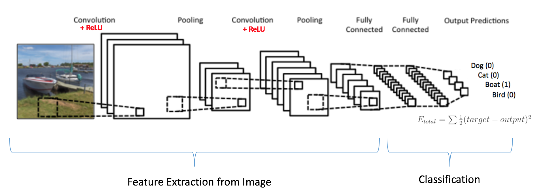
Figure 15: Training the ConvNet

The overall training process of the Convolution Network may be summarized as below:

• Step1: We initialize all filters and parameters / weights with random values

• Step2: The network takes a training image as input, goes through the forward propagation step (convolution, ReLU and pooling operations along with forward propagation in the Fully Connected layer) and finds the output probabilities for each class.
  • Lets say the output probabilities for the boat image above are [0.2, 0.4, 0.1, 0.3]
  • Since weights are randomly assigned for the first training example, output probabilities are also random.

• Step3: Calculate the total error at the output layer (summation over all 4 classes)
  •  Total Error = ∑  ½ (target probability – output probability) ²

• Step4: Use Backpropagation to calculate the gradients of the error with respect to all weights in the network and use gradient descent to update all filter values / weights and parameter values to minimize the output error.
  • The weights are adjusted in proportion to their contribution to the total error.
  • When the same image is input again, output probabilities might now be [0.1, 0.1, 0.7, 0.1], which is closer to the target vector [0, 0, 1, 0].
  • This means that the network has learnt to classify this particular image correctly by adjusting its weights / filters such that the output error is reduced.
  • Parameters like number of filters, filter sizes, architecture of the network etc. have all been fixed before Step 1 and do not change during training process – only the values of the filter matrix and connection weights get updated.

• Step5: Repeat steps 2-4 with all images in the training set.

The above steps train the ConvNet – this essentially means that all the weights and parameters of the ConvNet have now been optimized to correctly classify images from the training set.

When a new (unseen) image is input into the ConvNet, the network would go through the forward propagation step and output a probability for each class (for a new image, the output probabilities are calculated using the weights which have been optimized to correctly classify all the previous training examples). If our training set is large enough, the network will (hopefully) generalize well to new images and classify them into correct categories.

Note 1: The steps above have been oversimplified and mathematical details have been avoided to provide intuition into the training process. See [4] and [12] for a mathematical formulation and thorough understanding.

Note 2: In the example above we used two sets of alternating Convolution and Pooling layers. Please note however, that these operations can be repeated any number of times in a single ConvNet. In fact, some of the best performing ConvNets today have tens of Convolution and Pooling layers! Also, it is not necessary to have a Pooling layer after every Convolutional Layer. As can be seen in the Figure 16 below, we can have multiple Convolution + ReLU operations in succession before a having a Pooling operation. Also notice how each layer of the ConvNet is visualized in the Figure 16 below.

Figure 16: Source [4]

Visualizing Convolutional Neural Networks

In general, the more convolution steps we have, the more complicated features our network will be able to learn to recognize. For example, in Image Classification a ConvNet may learn to detect edges from raw pixels in the first layer, then use the edges to detect simple shapes in the second layer, and then use these shapes to deter higher-level features, such as facial shapes in higher layers [14]. This is demonstrated in Figure 17 below – these features were learnt using a Convolutional Deep Belief Network and the figure is included here just for demonstrating the idea (this is only an example: real life convolution filters may detect objects that have no meaning to humans).

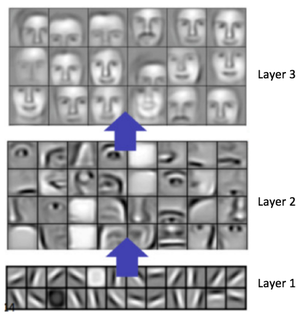
Figure 17: Learned features from a Convolutional Deep Belief Network

Adam Harley created amazing visualizations of a Convolutional Neural Network trained on the MNIST Database of handwritten digits [13]. I highly recommend playing around with it to understand details of how a CNN works.

We will see below how the network works for an input ‘8’. Note that the visualization in Figure 18 does not show the ReLU operation separately.

Figure 18: Visualizing a ConvNet trained on handwritten digits

The input image contains 1024 pixels (32 x 32 image) and the first Convolution layer (Convolution Layer 1) is formed by convolution of six unique 5 × 5 (stride 1) filters with the input image. As seen, using six different filters produces a feature map of depth six.

Convolutional Layer 1 is followed by Pooling Layer 1 that does 2 × 2 max pooling (with stride 2) separately over the six feature maps in Convolution Layer 1. You can move your mouse pointer over any pixel in the Pooling Layer and observe the 4 x 4 grid it forms in the previous Convolution Layer (demonstrated in Figure 19). You’ll notice that the pixel having the maximum value (the brightest one) in the 4 x 4 grid makes it to the Pooling layer.

Figure 19: Visualizing the Pooling Operation

Pooling Layer 1 is followed by sixteen 5 × 5 (stride 1) convolutional filters that perform the convolution operation. This is followed by Pooling Layer 2 that does 2 × 2 max pooling (with stride 2). These two layers use the same concepts as described above.

We then have three fully-connected (FC) layers. There are:

• 120 neurons in the first FC layer
• 100 neurons in the second FC layer
• 10 neurons in the third FC layer corresponding to the 10 digits – also called the Output layer

Notice how in Figure 20, each of the 10 nodes in the output layer are connected to all 100 nodes in the 2nd Fully Connected layer (hence the name Fully Connected).

Also, note how the only bright node in the Output Layer corresponds to ‘8’ – this means that the network correctly classifies our handwritten digit (brighter node denotes that the output from it is higher, i.e. 8 has the highest probability among all other digits).

Figure 20: Visualizing the Filly Connected Layers

The 3d version of the same visualization is available here.

Other ConvNet Architectures

Convolutional Neural Networks have been around since early 1990s. We discussed the LeNet above which was one of the very first convolutional neural networks. Some other influential architectures are listed below [3] [4].

• LeNet (1990s): Already covered in this article.

• 1990s to 2012: In the years from late 1990s to early 2010s convolutional neural network were in incubation. As more and more data and computing power became available, tasks that convolutional neural networks could tackle became more and more interesting.

• AlexNet (2012) – In 2012, Alex Krizhevsky (and others) released AlexNet which was a deeper and much wider version of the LeNet and won by a large margin the difficult ImageNet Large Scale Visual Recognition Challenge (ILSVRC) in 2012. It was a significant breakthrough with respect to the previous approaches and the current widespread application of CNNs can be attributed to this work.

• ZF Net (2013) – The ILSVRC 2013 winner was a Convolutional Network from Matthew Zeiler and Rob Fergus. It became known as the ZFNet (short for Zeiler & Fergus Net). It was an improvement on AlexNet by tweaking the architecture hyperparameters.

• GoogLeNet (2014) – The ILSVRC 2014 winner was a Convolutional Network from Szegedy et al. from Google. Its main contribution was the development of an Inception Module that dramatically reduced the number of parameters in the network (4M, compared to AlexNet with 60M).

• VGGNet (2014) – The runner-up in ILSVRC 2014 was the network that became known as the VGGNet. Its main contribution was in showing that the depth of the network (number of layers) is a critical component for good performance.

• ResNets (2015) – Residual Network developed by Kaiming He (and others) was the winner of ILSVRC 2015. ResNets are currently by far state of the art Convolutional Neural Network models and are the default choice for using ConvNets in practice (as of May 2016).

• DenseNet (August 2016) – Recently published by Gao Huang (and others), the Densely Connected Convolutional Network has each layer directly connected to every other layer in a feed-forward fashion. The DenseNet has been shown to obtain significant improvements over previous state-of-the-art architectures on five highly competitive object recognition benchmark tasks. Check out the Torch implementation here.

Conclusion

In this post, I have tried to explain the main concepts behind Convolutional Neural Networks in simple terms. There are several details I have oversimplified / skipped, but hopefully this post gave you some intuition around how they work.

This post was originally inspired from Understanding Convolutional Neural Networks for NLP by Denny Britz (which I would recommend reading) and a number of explanations here are based on that post. For a more thorough understanding of some of these concepts, I would encourage you to go through the notes from Stanford’s course on ConvNets as well as other excellent resources mentioned under References below. If you face any issues understanding any of the above concepts or have questions / suggestions, feel free to leave a comment below.

All images and animations used in this post belong to their respective authors as listed in References section below.

References

1. Clarifai Home Page
2. Shaoqing Ren, et al, “Faster R-CNN: Towards Real-Time Object Detection with Region Proposal Networks”, 2015, arXiv:1506.01497 
3. Neural Network Architectures, Eugenio Culurciello’s blog
4. CS231n Convolutional Neural Networks for Visual Recognition, Stanford
5. Clarifai / Technology
6. Machine Learning is Fun! Part 3: Deep Learning and Convolutional Neural Networks
7. Feature extraction using convolution, Stanford
8. Wikipedia article on Kernel (image processing) 
9. Deep Learning Methods for Vision, CVPR 2012 Tutorial 
10. Neural Networks by Rob Fergus, Machine Learning Summer School 2015
11. What do the fully connected layers do in CNNs? 
12. Convolutional Neural Networks, Andrew Gibiansky 
13. A. W. Harley, “An Interactive Node-Link Visualization of Convolutional Neural Networks,” in ISVC, pages 867-877, 2015 (link)
14. Understanding Convolutional Neural Networks for NLP
15. Backpropagation in Convolutional Neural Networks
16. A Beginner’s Guide To Understanding Convolutional Neural Networks
17. Vincent Dumoulin, et al, “A guide to convolution arithmetic for deep learning”, 2015, arXiv:1603.07285
18. What is the difference between deep learning and usual machine learning?
19. How is a convolutional neural network able to learn invariant features?
20. A Taxonomy of Deep Convolutional Neural Nets for Computer Vision

Original post: Reposted with permission.

Bio: Ujjwal Karn has 3 years of industry and research experience in machine learning and is interested in practical applications of deep learning to language and vision understanding.

Related:

• Deep Learning cleans podcast episodes from ‘ahem’ sounds
• How Convolutional Neural Networks Work
• Deep Learning Key Terms, Explained