A Quick Introduction to Neural Networks

A feedforward neural network can consist of three types of nodes:

1. Input Nodes - The Input nodes provide information from the outside world to the network and are together referred to as the "Input Layer". No computation is performed in any of the Input nodes - they just pass on the information to the hidden nodes.
2. Hidden Nodes - The Hidden nodes have no direct connection with the outside world (hence the name "hidden"). They perform computations and transfer information from the input nodes to the output nodes. A collection of hidden nodes forms a "Hidden Layer". While a feedforward network will only have a single input layer and a single output layer, it can have zero or multiple Hidden Layers.
3. Output Nodes - The Output nodes are collectively referred to as the "Output Layer" and are responsible for computations and transferring information from the network to the outside world.

In a feedforward network, the information moves in only one direction - forward - from the input nodes, through the hidden nodes (if any) and to the output nodes. There are no cycles or loops in the network [3] (this property of feed forward networks is different from Recurrent Neural Networks in which the connections between the nodes form a cycle).

Two examples of feedforward networks are given below:

1. Single Layer Perceptron - This is the simplest feedforward neural network [4] and does not contain any hidden layer. You can learn more about Single Layer Perceptrons in [4], [5], [6], [7].

2. Multi Layer Perceptron - A Multi Layer Perceptron has one or more hidden layers. We will only discuss Multi Layer Perceptrons below since they are more useful than Single Layer Perceptons for practical applications today.

Multi Layer Perceptron

A Multi Layer Perceptron (MLP) contains one or more hidden layers (apart from one input and one output layer). While a single layer perceptron can only learn linear functions, a multi layer perceptron can also learn non - linear functions.

Figure 4 shows a multi layer perceptron with a single hidden layer. Note that all connections have weights associated with them, but only three weights (w0, w1, w2) are shown in the figure.

Input Layer: The Input layer has three nodes. The Bias node has a value of 1. The other two nodes take X1 and X2 as external inputs (which are numerical values depending upon the input dataset). As discussed above, no computation is performed in the Input layer, so the outputs from nodes in the Input layer are 1, X1 and X2 respectively, which are fed into the Hidden Layer.

Hidden Layer: The Hidden layer also has three nodes with the Bias node having an output of 1. The output of the other two nodes in the Hidden layer depends on the outputs from the Input layer (1, X1, X2) as well as the weights associated with the connections (edges). Figure 4 shows the output calculation for one of the hidden nodes (highlighted). Similarly, the output from other hidden node can be calculated. Remember that f refers to the activation function. These outputs are then fed to the nodes in the Output layer.

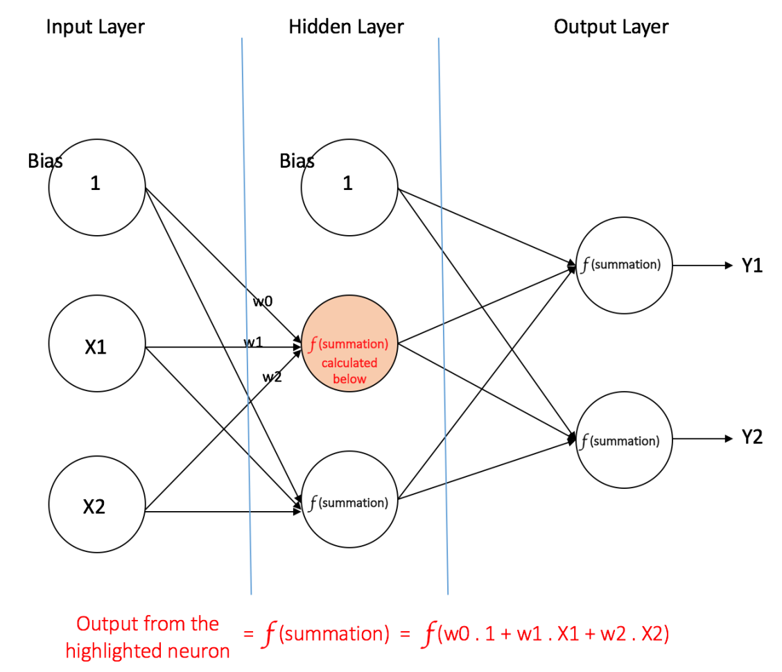
Figure 4: a multi layer perceptron having one hidden layer

Output Layer: The Output layer has two nodes which take inputs from the Hidden layer and perform similar computations as shown for the highlighted hidden node. The values calculated (Y1 and Y2) as a result of these computations act as outputs of the Multi Layer Perceptron.

Given a set of features X = (x1, x2, ...) and a target y, a Multi Layer Perceptron can learn the relationship between the features and the target, for either classification or regression.

Lets take an example to understand Multi Layer Perceptrons better. Suppose we have the following student-marks dataset:

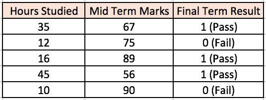
The two input columns show the number of hours the student has studied and the mid term marks obtained by the student. The Final Result column can have two values 1 or 0 indicating whether the student passed in the final term. For example, we can see that if the student studied 35 hours and had obtained 67 marks in the mid term, he / she ended up passing the final term.

Now, suppose, we want to predict whether a student studying 25 hours and having 70 marks in the mid term will pass the final term.

This is a binary classification problem where a multi layer perceptron can learn from the given examples (training data) and make an informed prediction given a new data point. We will see below how a multi layer perceptron learns such relationships.

Training our MLP: The Back-Propagation Algorithm

The process by which a Multi Layer Perceptron learns is called the Backpropagation algorithm. I would recommend reading this Quora answer by Hemanth Kumar (quoted below) which explains Backpropagation clearly.

Backward Propagation of Errors, often abbreviated as BackProp is one of the several ways in which an artificial neural network (ANN) can be trained. It is a supervised training scheme, which means, it learns from labeled training data (there is a supervisor, to guide its learning).

To put in simple terms, BackProp is like "learning from mistakes". The supervisor corrects the ANN whenever it makes mistakes.

An ANN consists of nodes in different layers; input layer, intermediate hidden layer(s) and the output layer. The connections between nodes of adjacent layers have "weights" associated with them. The goal of learning is to assign correct weights for these edges. Given an input vector, these weights determine what the output vector is.

In supervised learning, the training set is labeled. This means, for some given inputs, we know the desired/expected output (label).

BackProp Algorithm:
Initially all the edge weights are randomly assigned. For every input in the training dataset, the ANN is activated and its output is observed. This output is compared with the desired output that we already know, and the error is "propagated" back to the previous layer. This error is noted and the weights are "adjusted" accordingly. This process is repeated until the output error is below a predetermined threshold.

Once the above algorithm terminates, we have a "learned" ANN which, we consider is ready to work with "new" inputs. This ANN is said to have learned from several examples (labeled data) and from its mistakes (error propagation).

Now that we have an idea of how Backpropagation works, lets come back to our student-marks dataset shown above.