ResNets, HighwayNets, and DenseNets, Oh My!
This post walks through the logic behind three recent deep learning architectures: ResNet, HighwayNet, and DenseNet. Each make it more possible to successfully trainable deep networks by overcoming the limitations of traditional network design.
By Arthur Juliani, University of Oregon.

When it comes to neural network design, the trend in the past few years has pointed in one direction: deeper. Whereas the state of the art only a few years ago consisted of networks which were roughly twelve layers deep, it is now not surprising to come across networks which are hundreds of layers deep. This move hasn’t just consisted of greater depth for depths sake. For many applications, the most prominent of which being object classification, the deeper the neural network, the better the performance. That is, provided they can be properly trained! In this post I would like to walk through the logic behind three recent deep learning architectures: ResNet, HighwayNet, and DenseNet. Each make it more possible to successfully trainable deep networks by overcoming the limitations of traditional network design. I will also be providing Tensorflow code to easily implement each of these networks. If you’d just like the code, you can find that here. Otherwise, read on!
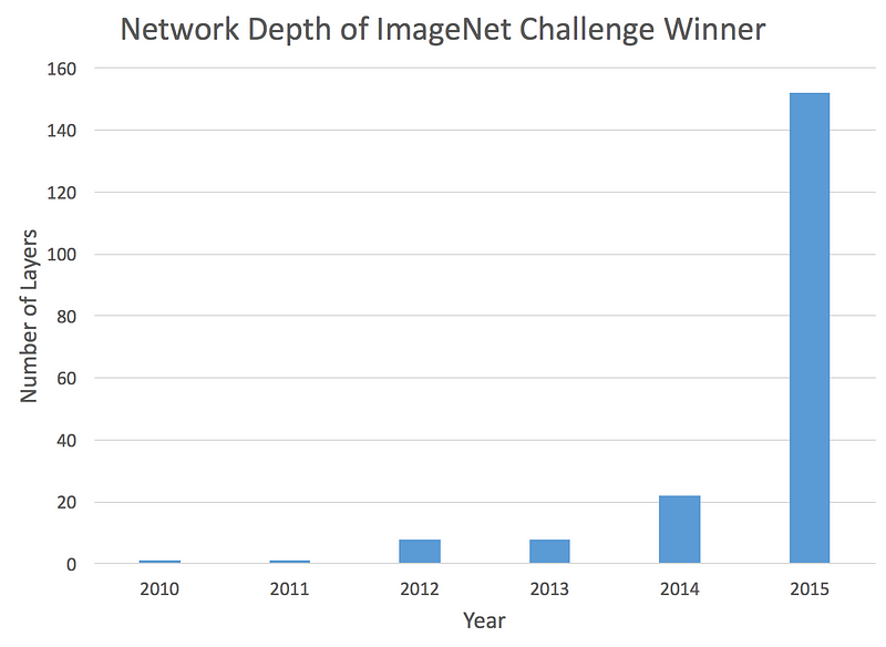
The trend toward deeper networks is clear.
Why Naively Going Deeper Doesn’t Work
The first intuition when designing a deep network may be to simply stack many of the typical building blocks such as convolutional or fully-connected layers together. This works to a point, but performance quickly diminishes the deeper a traditional network becomes. The issue arises from the way in which neural networks are trained through backpropogation. When a network is being trained, a gradient signal must be propagated backwards through the network from the top layer all the way down to the bottom most layer in order to ensure that the network updates itself appropriately. With a traditional network this gradient becomes slightly diminished as it passes through each layer of the network. For a network with just a few layers, this isn’t an issue. For a network with more than a couple dozen layers however, the signal essentially disappears by the time it reaches the beginning of the network again.
So the problem is to design a network in which the gradient can more easily reach all the layers of a network which might be dozens, or even hundreds of layers deep. This is the goal behind the following state of the art architectures: ResNets, HighwayNets, and DenseNets.
Residual Network
A Residual Network, or ResNet is a neural network architecture which solves the problem of vanishing gradients in the simplest way possible. If there is trouble sending the gradient signal backwards, why not provide the network with a shortcut at each layer to make things happen more smoothly? In a traditional network the activation at a layer is defined as follows:
y = f(x)
Where f(x) is our convolution, matrix multiplication, or batch normalization, etc. When the signal is sent backwards, the gradient always must pass through f(x), which can cause trouble due to the nonlinearities which are involved. Instead, at each layer the ResNet implements:
y = f(x) + x
The “+ x” at the end is the shortcut. It allows the gradient to pass backwards directly. By stacking these layers, the gradient could theoretically “skip” over all the intermediate layers and reach the bottom without being diminished.
While this is the intuition, the actual implementation is a little more complex. In the latest incarnation of ResNets, f(x) + x takes the form:
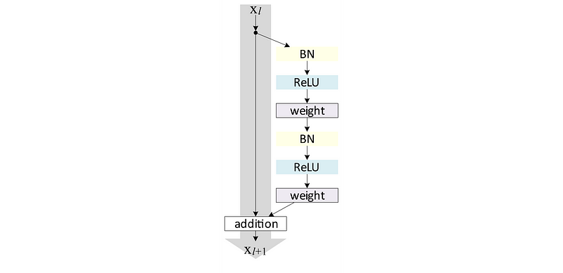
With Tensorflow we can implement a network composed of these Residual units as follows:
Highway Network
The second architecture I’d like to introduce is the Highway Network. It builds on the ResNet in a pretty intuitive way. The Highway Network preserves the shortcuts introduced in the ResNet, but augments them with a learnable parameter to determine to what extent each layer should be a skip connection or a nonlinear connection. Layers in a Highway Network are defined as follows:

In this equation we can see an outline of the previous two kinds of layers discussed: y = H(x,Wh) mirrors our traditional layer, and y = H(x,Wh) + x mirrors our residual unit. What is new is the T(x,Wt) function. This serves at the switch to determine to what extent information should be sent through the primary pathway or the skip pathway. By using T and (1-T) for each of the two pathways, the activation must always sum to 1. We can implement this in Tensorflow as follows:
Dense Networks
Finally I want to introduce the Dense Network, or DenseNet. You might say that is architecture takes the insights of the skip connection to the extreme. The idea here is that if connecting a skip connection from the previous layer improves performance, why not connect every layer to every other layer? That way there is always a direct route for the information backwards through the network.
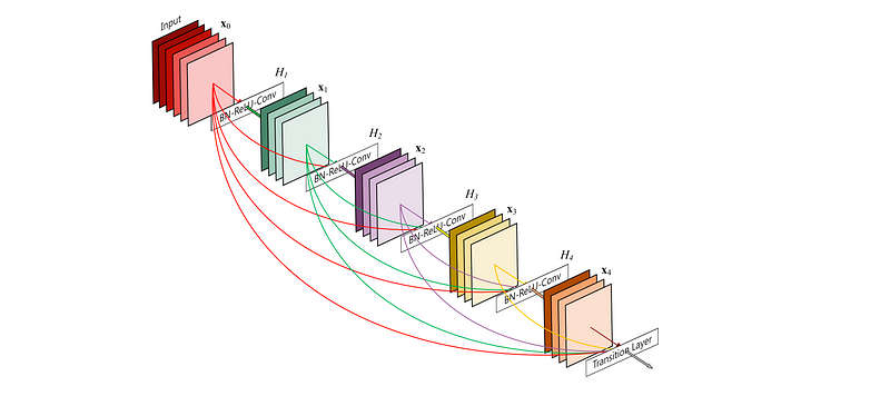
Instead of using an addition however, the DenseNet relies on stacking of layers. Mathematically this looks like:
y = f(x,x-1,x-2... x-n)
This architecture makes intuitive sense in both the feedforward and feed backward settings. In the feed-forward setting, a task may benefit from being able to get low-level feature activations in addition to high level feature activations. In classifying objects for example, a lower layer of the network may determine edges in an image, whereas a higher layer would determine larger-scale features such as presence of faces. There may be cases where being able to use information about edges can help in determining the correct object in a complex scene. In the backwards case, having all the layers connected allows us to quickly send gradients to their respective places in the network easily.
When implementing DenseNets, we can’t just connected everything though. Only layers with the same height and width can be stacked. So we instead densely stack a set of convolutional layers, then apply a striding or pooling layer, then densely stack another set of convolutional layers, etc. This can be implemented in Tensorflow as follows:
All of these network can be trained to classify images using the CIFAR10 dataset, and can perform well with dozens of layers where a traditional neural network fails. With little parameter tuning I was able to get them to perform above 90% accuracy on a test set after only an hour or so. The full code for training each of these models, and comparing them to a traditional networks is available here. I hope this walkthrough has been a helpful introduction to the world of really deep neural networks!
If you’d like to follow my work on Deep Learning, AI, and Cognitive Science, follow me on Medium @Arthur Juliani, or on twitter @awjliani.
Bio: Arthur Juliani is a researcher working at the intersection of Cognitive Neuroscience and Deep Learning. He is currently obtaining his Phd from the University of Oregon, and enjoys writing about AI in his free time
Original. Reposted with permission.
Related: