 Deep Learning Research Review: Natural Language Processing
 Deep Learning Research Review: Natural Language Processing
This edition of Deep Learning Research Review explains recent research papers in Natural Language Processing (NLP). If you don't have the time to read the top papers yourself, or need an overview of NLP with Deep Learning, this post is for you.
Recurrent Neural Networks (RNNs)
Okay, so now that we have our word vectors, let’s see how they fit into recurrent neural networks. RNNs are the go-to for most NLP tasks today. The big advantage of the RNN is that it is able to effectively use data from previous time steps. This is what a small piece of an RNN looks like.
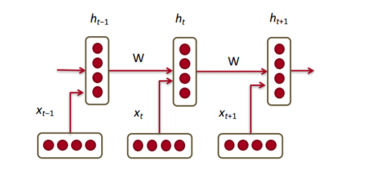
So, at the bottom we have our word vectors (xt, xt-1, xt+1). Each of the vectors has a hidden state vector at that same time step (ht, ht-1, ht+1). Let’s call this one module.
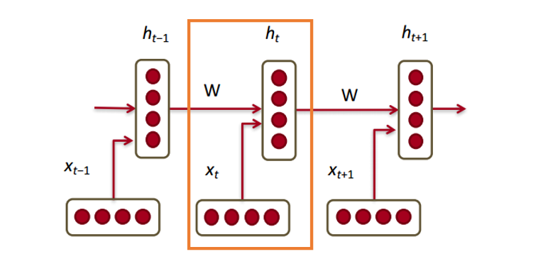
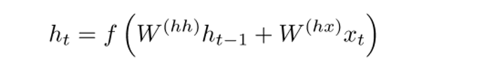
The hidden state in each module of the RNN is a function of both the word vector and the hidden state vector at the previous time step.
If you take a close look at the superscripts, you’ll see that there’s a weight matrix Whx which we’re going to multiply with our input, and there’s a recurrent weight matrix Whh which is multiplied with the hidden state vector at the previous time step. Keep in mind that these recurrent weight matrices are the same across all time steps. This is the key point of RNNs. Thinking about this carefully, it’s very different from a traditional 2 layer NN for example. In that case, we normally have a distinct W matrix for each layer (W1 and W2). Here, the recurrent weight matrix is the same through the network.
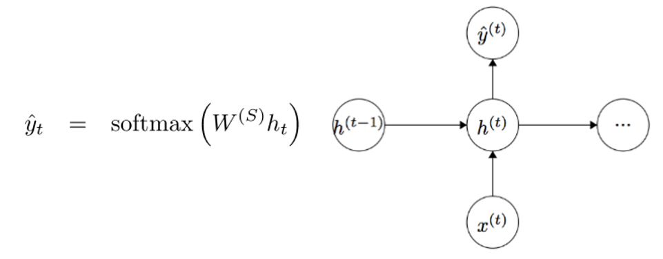
To get the output (Yhat) of a particular module, this will be h times WS, which is another weight matrix.
Let’s take a step back now and understand what the advantages of an RNN are. The most distinct difference from a traditional NN is that an RNN takes in a sequence of inputs (words in our case). You can contrast this to a typical CNN where you’d have just a singular image as input. With an RNN, however, the input can be anywhere from a short sentence to a 5 paragraph essay. Additionally, the order of inputs in this sequence can largely affect how the weight matrices and hidden state vectors change during training. The hidden states, after training, will hopefully capture the information from the past (the previous time steps).
Gated Recurrent Units (GRUs)
Let’s now look at a gated recurrent unit, or GRU. The purpose of this unit is to provide a more complex way of computing our hidden state vectors in RNNs. This approach will allow us to keep information that capture long distance dependencies. Let’s imagine why long term dependencies would be a problem in the traditional RNN setup. During backpropagation, the error will flow through the RNN, going from the latest time step to the earliest one. If the initial gradient is a small number (say < 0.25), then by the 3rd or 4th module, the gradient will have practically vanished (chain rule multiplies gradients together) and thus the hidden states of the earlier time steps won’t get updated.
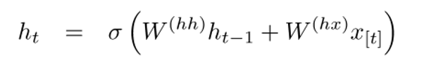
In a traditional RNN, the hidden state vector is computed through this formulation.
The GRU provides a different way of computing this hidden state vector h(t). The computation is broken up into 3 components, an update gate, a reset gate, and a new memory container. The two gates are both functions of the input word vector and the hidden state at the previous time step.
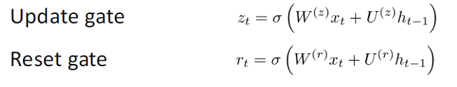
The key difference is that different weights are used for each gate. This is indicated by the differing superscripts. The update gate uses Wz and Uz while the reset gate uses Wr and Ur.
Now, the new memory container is computed through the following.
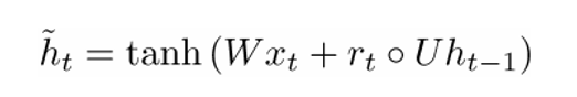
(The open dot indicates a Hadamard product)
Now, if you take a closer look at the formulation, you’ll see that if the reset gate unit is close to 0, then that whole term becomes 0 as well, thus ignoring the information in ht-1 from the previous time steps. In this scenario, the unit is only a function of the new word vector xt.
The final formulation of h(t) is written as
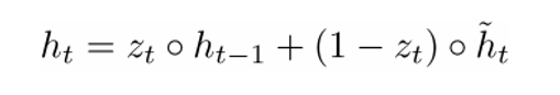
ht is a function of all 3 components: the reset gate, the update gate, and the memory container. The best way to understand this is by visualizing what happens when zt is close to 1 and when it is close to 0. When zt is close to 1, the new hidden state vector htis mostly dependent on the previous hidden state and we ignore the current memory container because (1-zt) goes to 0. When ztis close to 0, the new hidden state vector ht is mostly dependent on the current memory container and we ignore the previous hidden state. An intuitive way of looking at these 3 components can be summarized through the following.
- Update Gate:
- If zt ~ 1, then ht completely ignores the current word vector and just copies over the previous hidden state (If this doesn’t make sense, look at the ht equation and take note of what happens to the 1 - zt term when zt ~ 1).
- If zt ~ 0, then ht completely ignores the hidden state at the previous time step and is dependent on the new memory container.
- This gate lets the model control how much of the information in the previous hidden state should influence the current hidden state.
- Reset Gate:
- If rt ~ 1, then the memory container keeps the info from the previous hidden state.
- If rt ~ 0, then the memory container ignores the previous hidden state.
- This gate lets the model drop information if that info is irrelevant in the future.
- Memory Container: Dependent on the reset gate.
A common example to illustrate the effectiveness of GRUs is the following. Let’s say you have the following passage.

and the associated question “What is the sum of the 2 numbers?”. Since the middle sentence has absolutely no impact on the question at hand, the reset and update gates will allow the network to “forget” the middle sentence in some sense, and learn that only specific information (numbers in this case) should modify the hidden state.
Long Short Term Memory Units (LSTMs)
If you’re comfortable with GRUs, then LSTMs won’t be too far of a leap forward. An LSTM is also made up of a series of gates.
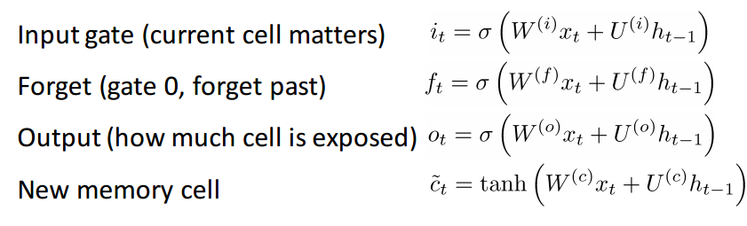
Definitely a lot more information to take in. Since this can be thought of as an extension to the idea behind a GRU, I won’t go too far into the analysis, but for a more in depth walkthrough of each gate and each piece of computation, check out Chris Olah’s amazingly well written blog post. It is by far, the most popular tutorial on LSTMs, and will definitely help those of you looking for more intuition as to why and how these units work so well.
Comparing and Contrasting LSTMs and GRUs
Let’s start off with the similarities. Both of these units have the special function of being able to keep long term dependencies between words in a sequence. Long term dependencies refer to situations where two words or phrases may occur at very different time steps, but the relationship between them is still critical to solving the end goal. LSTMs and GRUs are able to capture these dependencies through gates that can ignore or keep certain information in the sequence.
The difference between the two units lies in the number of gates that they have (GRU – 2, LSTM – 3). This affects the number of nonlinearities the input passes through and ultimately affects the overall computation. The GRU also doesn’t have the same memory cell (ct) that the LSTM has.
Before Getting Into the Papers
Just want to make one quick note. There are a couple other deep models that are useful in NLP. Recursive neural networks and CNNs for NLP are sometimes used in practice, but aren’t as prevalent as RNNs, which really are the backbone behind most deep learning NLP systems.
Alright. Now that we have a good understanding of deep learning in relation to NLP, let’s look at some papers. Since there are numerous different problem areas within NLP (from machine translation to question answering), there are a number of papers that we could look into, but here are 3 that I found to be particularly insightful. 2016 had some great advancements in NLP, but let’s first start with one from 2015.