Applying Machine Learning To March Madness
March Madness is upon us. But before you get your brackets set, check out this overview of using machine learning to do the heavy lifting for you. A great discussion, and a timely topic.
Introduction
March. Madness.
The two words that can send goosebumps to every college basketball fan in the country. It’s the month where every fan will fill out a bracket, each thinking that they picked the right 12 over 5 seed upset or that they were the only one to pick the Cinderella team that makes it to the Elite 8. The month where people will spend hours watching regular season games, pouring over stats and expert analysis, trying to carefully predict the most likely winner, only to find their pick lose in the first round (Thanks Michigan State ). The month where your younger sister ends up having a better bracket than you because she picked the teams with the “cooler” mascots (Sad, but true story). March Madness is the sports phenomenon that incites anxiety, regret, elation, and every other possible emotion in the spectrum. And it’s about to start in 4 days.
Never heard of it?
March Madness refers to the annual collegiate men's basketball tournament. The tournament is made up of 64 college teams competing in a single elimination format. In order to win the championship, a team has to win 6 consecutive games.
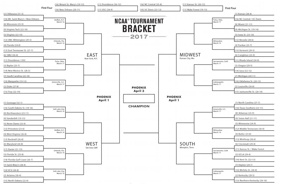
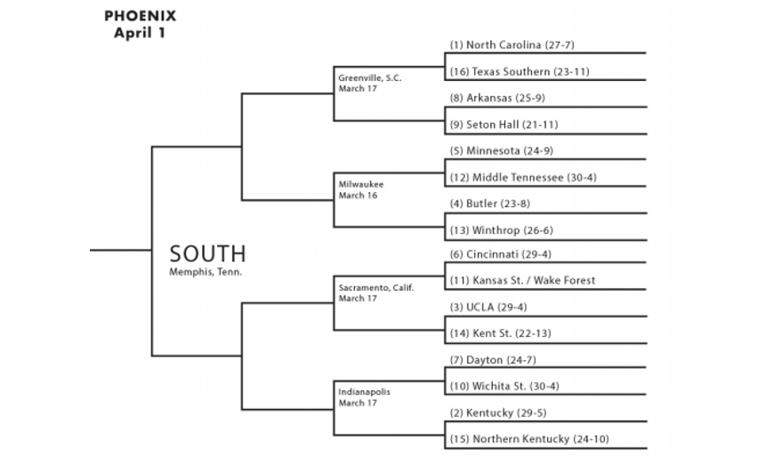
The tournament is broken up into 4 regions. Each region has 16 teams, ranked from 1 to 16. This ranking is determined by a NCAA committee and is based on each team’s regular season performance. The NCAA structures the games so that the highest seed in a region plays the lowest seed, the 2nd highest plays the 2nd lowest, and so on.
So, what’s the big deal?
One in 9.2 quintillion.
Those are the odds that you will correctly pick the winners of all 63 games played over the course of the tournament. Mathematically speaking, there are 263 (~ 9.2 quintillion) number of ways that you can fill the bracket. In 2014, Warren Buffet famously offered 1 billion dollars to anyone who could fill out a perfect bracket (Needless to say, nobody even really came close).
As sports fans, predicting the outcomes of games is in our nature. We want to believe our alma mater will make it to the Sweet Sixteen. We want to have the bragging rights of saying that we knew 11th seed VCU would make it to the Final Four (2011 was insane). The allure of March Madness comes through the unpredictable nature of such a large single elimination tournament. While it could be easy for one to just pick all of the number 1 seeds to advance (this is known as picking “chalk”), tournament history says that there are going to be more than a few surprises.
Throughout the next 2 weeks, fans will be streaming games in class (personal experience) or at work, watching incredible buzzer-beaters, mind-blowing upsets, and most importantly, hoping that their bracket doesn’t get busted within the first day.
The Prediction Problem
Before getting into machine learning, let’s take a step back and think about the idea of sports game prediction. Not a very complex topic right? Imagine this situation.
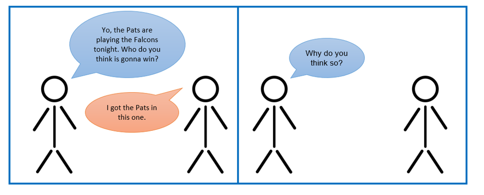
Let’s stop the situation right there. The fundamental question in sports prediction arises: What factors do you, as the predictor, use in determining the outcome of a future sporting event? Imagine the types of responses you might get.
Person A: “The Pats have the best defense in the NFL according to points allowed per game, they have the 4th fewest rushing yards allowed, and are the 3rd best in the league in turnover differential. They’ll win easily.”
Person B: “72 out of the 100 NFL ESPN analysts picked the Pats, so Imma go with them.
Person C: “The Pats have Tom Brady and I like Tom Brady.”
Person D: “My ex-girlfriend likes the Falcons, so go Pats!”
As you look at each of these responses, you’ll see that each response places a different importance (“weight” in ML terms) on a particular stat/feeling/emotion (“feature” in ML terms). Person A relied heavily upon regular season statistics to make a prediction. Person B chose to take into account the opinions of the NFL analysts at ESPN. Person C showed a personal preference toward Tom Brady, causing him/her to choose the Patriots. Finally, Person D might have never watched a football game before, but chose the Patriots because of negative sentiments towards a particular person.
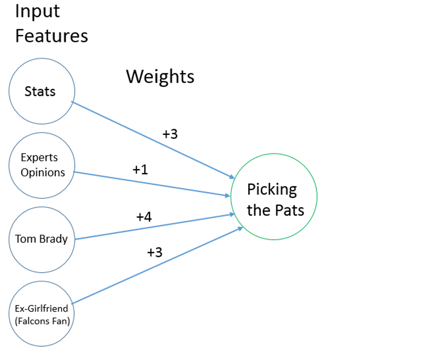
The bottom-line is that we all have different ways of making predictions. We all have different input features that we consider, we all have different weights placed on them, and thus we all have different ways of interpreting how a future sports matchup will play out.
Having all of these different viewpoints towards prediction is great. It’s what allows us to have those intense disagreements before the game, and what allows us to bask in the glory of bragging rights or cause us to rethink our predictive thought process.
The one commonality in all of our viewpoints is that we are biased. There’s no 2 ways about it. Each and every one of us is biased in the way that we approach sports prediction. We’re biased because there’s no clear cut answer to the question of “What makes a good prediction?”. Should we look at stats? Should we pay attention to intangibles? Should we just forget all of that and simply make predictions based on personal feelings? There isn’t an easy solution.
That’s where machine learning comes in.
Can Machine Learning Help With Predictions?
Okay, so with the last paragraph, we’ve established the problem space. We want to see if we can build an ML model that is able to look at training data (past NCAA basketball games), find the relationship between a team’s success and their attributes (stats), and output predictions for future games.
So, why can machine learning be a possible use case for this prediction problem? Well, first of all, the data is there. We have a bunch of it. Over 100,000 NCAA regular season games were played over the last 25+ years, and we generally have plenty of statistics about the teams for each season. Because we have all of this data, we can try to use machine learning to find out what particular statistics most correlate with a team winning a particular matchup. If a team allows less than 60 PPG, are they more likely to win the game? If a team turns the ball over more than 15 times, is that a fatal sign that they’ll lose to a team that does care of the ball? These are the types of questions that we hope data analysis and machine learning can lend insight to.
All the code for this data analysis can be found in this iPython Notebook. Be sure to follow along!
Basic Model Structure
Our ML model will take in information about two teams (Team 1 and Team 2) as input, and then output a probability of Team 1 winning that matchup.
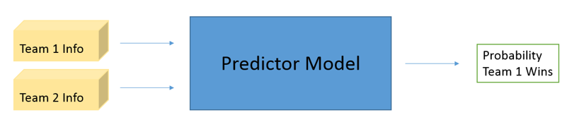
Now, the immediate problem that comes to mind is that ML algorithms normally have inputs in the form of singular matrices or vectors. We need to think of a way of encapsulating information about both teams in a single vector. Let’s first see if we can represent each team as a vector first.
Take the 2016 Kansas Jayhawks for example.
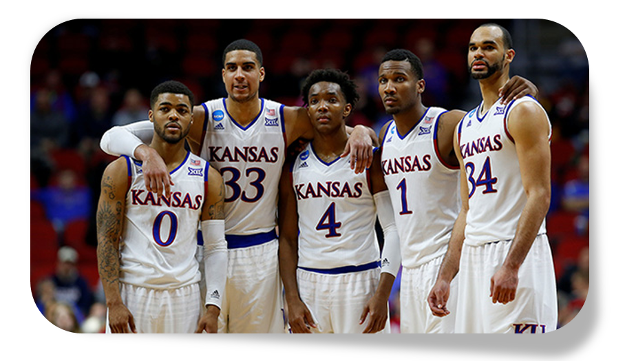
The Jayhawks had a great season, winning their 12th straight Big 12 title and getting a #1 seed in the tournament. Let’s think about how to represent their season in a single vector. In ML terms, what features do we want to represent? Let’s start with common statistical measures.
- Number of regular season wins: 29
- Average Points Per Game Scored: 80.30
- Average Points Per Game Allowed: 67.61
- Average 3’s Per Game Made: 9.21
- Average Turnovers Per Game: 14.39
- Average Assists Per Game: 18.30
- Average Rebounds Per Game: 43.73
- Average Steals Per Game: 7.66
Then, we can think about other factors related to the conference they played in.
- “Power 6” Conference (Big 12, Big 10, SEC, ACC, Pac-12, Big East): 1 - Binary Label
- Regular Season Conference Championship: 1 - Binary Label
- Conference Tournament Championship: 1 - Binary Label
We can consider other more advanced metrics.
- Simple Rating System (Function of strength of schedule and average point differential): 23.87
- Strength of Schedule: 11.22
Finally, we also look at some historical factors.
- Number of tournament appearances since 1985: 31
- Number of national championships since 1985: 2
Lastly, we have one ternary label that describes the location.
- Location (-1 for if Team 1 is away, 0 for neutral, and 1 for if Team 1 is home): 1
To create our representation for the 2016 Kansas Jayhawks, we can just concatenate all the features into a 16 dimensional vector.

Now, let’s do the same with another team from the 2016 season, the Oklahoma Sooners.

The Sooners, led by NBA first round draft pick Buddy Hield, had an incredible season, winning 25 games in the regular season, and coming away with a #2 seed in the tourney. We can see Oklahoma’s vector below.

We can think of coming up with team vectors as similar to the idea of using word vectors in deep learning approaches to NLP. Before feeding the input through a RNN or LSTM, we first have to transform our sentence or phrase into a usable representation.
Looking at the task of sports game prediction, let’s think about what we want our model to do. Since ML models normally take a single input, we can represent each matchup as the difference between the two team vectors (Team 1 vector - Team 2 vector). This is one way of representing the matchup. While some may choose to concatenate the two vectors instead, taking the difference helps to emphasize the ways that the teams are dissimilar from one another, which could help in determining the types of stats that are influential to the outcome of a matchup.
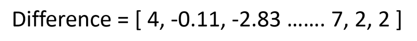
Our model will take in this difference vector, and output the probability that Team 1 wins the matchup.
The way that we train this model is by looking at the outcomes of past regular season games, and by looking at the team vectors of the two competing teams. Let’s take a look an actual training example to make this clearer.
Oklahoma and Kansas met twice in the 2016 regular season. The first meeting, played at the famous Allen Fieldhouse in Kansas, ended up being one of the greatest college basketball regular season games of all time.
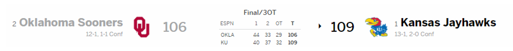
#1 vs #2. Triple Overtime. Yeah, that game was intense. It’s going to be one of many games in our training data. How will this particular game look like?
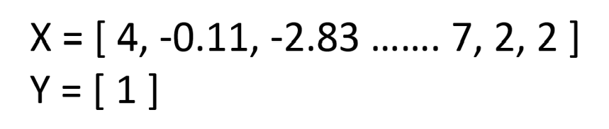
Make sense? The X component of every training example will be the difference between the two team vectors for that season. The Y component of the training example will be either [1] or [0], representing if Team 1 won or if Team 2 won, respectively.
The Kaggle dataset and stats from Sports-Reference had regular season and tournament data from the 1993 season onwards. From 1993 to 2016, there were over 115,000 games played. Our dimensionality for xTrain will be 115113 x 16 and 115113 x 1 for yTrain.
Applying ML Algorithms
Now that we have our training set, we have to choose an ML algorithm. From simple logistic regression to random forests to complex ensembles, there’s a variety of models that could fit our task.
Whenever you’re first starting out with a dataset and a prediction task, always try out a very simple model (e.g Linear/Logistic Regression or Decision Trees or KNN) before experimenting with more complex neural network and ensemble approaches. After splitting the training data into train and sets, we train the model (using Scikit-Learn functions), and evaluate it on the test set.
Below, you can see a table of how well a bunch of our models performed. To ensure that a model didn’t just get lucky with easy games to classify, we evaluated the models 100 times on different train/test splits and took the average.
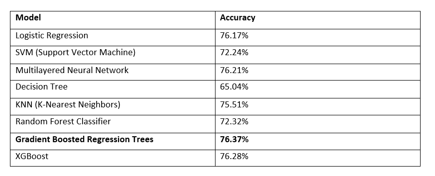
Gradient Boosted Trees
This model obtained the best performance on the test sets. This model is basically a type of ensemble network where you have multiple shallow regression or classification trees that reweight training examples based on the errors of the previous trees (If you’d like more info, check out Peter Prettenhofer’s great talk). Gradient boosted trees work really well with heterogeneous data (data on different scales) and can detect non-linear feature interactions, which was extremely useful in our task. One of the interesting attributes of this model is that we can analyze each of the feature’s importance to the overall classification. By looking at each feature in relation to its position on the regression trees, we can examine which features contributed the most to the correct classification of the games.
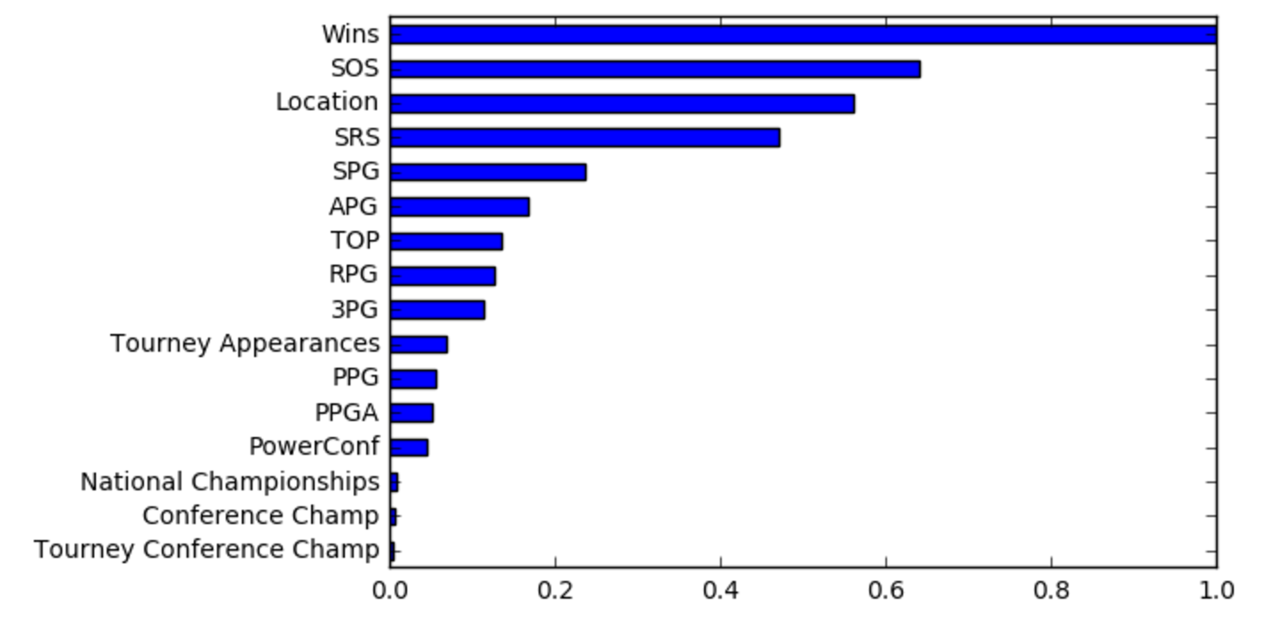
So, as you can see, the number of regular season wins that a team has greatly affects if they win the game or not. Intuitively, this makes sense. It doesn’t take an advanced ML model or an expert analyst to just predict that the team with the greater number of wins is more likely to win.
What’s interesting, however, is looking at the subsequent features in the list. The two features that follow are SOS (strength of schedule) and location. If you think about it, SOS makes intuitive sense as well. Even if a team doesn’t have a high number of wins, it’s still very possible that they are a great team that just played stronger opponents over the course of the season. Location is also a well known factor that influences games, as that is where the term “home-court advantage” comes from.
Next Steps
76.37% accuracy is great, but what can we do to really push it to 80 or 85 percent? Well, this is one of the tough parts of being an ML practitioner. There isn’t really a clear set of guidelines for improving your model. For decision trees, you can try increasing the depth of your tree. For neural networks, you can also try new architectures or the classic “just add another layer” mentality. There are infinitely many hyperparameters you can try to tune.
However, I’m going to focus more on the representation of the data, and the model itself. Here are a couple adjustments that could yield better results for next year’s tourney.
- In addition to relying on common statistical features (PPG, APG, etc), could try to quantify expert opinions, fan polls, or betting lines.
- Use SVD or PCA to reduce dimensionality and have the model learn to predict from a dataset with simpler features.
- Incorporate historical information about tournament results (e.g Number of times that the 12 seed wins over the 5 seed in a first round matchup)
- Experiment with different ways of consolidating the 2 team vectors into one (e.g concantenating, averaging, etc)
- Consider using a RNN type model that looks at time series data. Instead of representing a season as a single vector, could try to model a team’s progression as a time series. Thus, we’d be able to find out which teams are doing particularly well leading into the tournament.
Discussion of Bias in ML Models
I want to take a little bit of time right now to address an issue that I think is incredibly important for all machine learning practitioners. It’s the idea of training set bias. Like I mentioned in the beginning of the post, we’re all biased as human beings when it comes to prediction. In sports prediction, we have personal attachments to certain teams, incomplete views of the available statistics, and sometimes inconsistent criteria for judging matchups. Using machine learning allows us to leverage the huge amounts of data associated with prediction tasks. However, it still suffers from similar problems of bias that affect us.
The way bias affects ML models is through the training set we use and our representations (in this case, our team vectors). As ML practitioners, we make conscious decisions about what training data to use. For this particular model, I made the decision to use all of the regular season and tournament game data since 1993. I could have made the decision to include data from only the more recent years or I could have looked for datasets that had information on games before 1993.
Same with the features that I chose. I could have added features like Free Throw Percentage or Number of Home Wins, etc. But I didn’t. I created the features that I created because I believed that those were the most likely statistics that would correlate with a team’s success.
This type of control over the dataset and feature selection means that we have more responsibility over a model’s outputs than we think.
The main point is that ML models aren’t just pulling predictions out of nowhere. They are black boxes in a way, but it’s still up to us to decide what data we feed it and how we represent that data. While sports prediction is just a fun and benign task, there are many areas (healthcare, law, insurance, etc) where the results of machine learning models are incredibly important. We need to take time to make sure that the training data we use is representative of the whole population, doesn’t discriminate toward a group, and that the model is well fit to most examples in the both the training set and test sets.
ML Model 2017 Tournament Predictions
For the predictions for this year’s tournament, I ran a trained Gradient Boosted Classifier model on each of the first round games and had the team with the higher probability advance to the next round. I then repeated the process for all subsequent rounds.
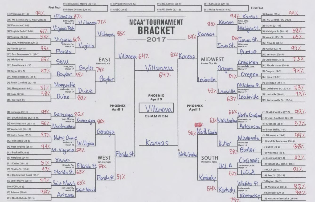
So, do you have your bracket ready?
Shout out to my good friend Arvind Sankar for helpful discussions on feature creation and for some of the data scraping scripts.
Bio: Adit Deshpande is currently a second year undergraduate student majoring in computer science and minoring in Bioinformatics at UCLA. He is passionate about applying his knowledge of machine learning and computer vision to areas in healthcare where better solutions can be engineered for doctors and patients.
Original. Reposted with permission.
Related: