Building, Training, and Improving on Existing Recurrent Neural Networks
In this post, we’ll provide a short tutorial for training a RNN for speech recognition, including code snippets throughout.
By Matthew Rubashkin & Matt Mollison, Silicon Valley Data Science.

On the deep learning R&D team at SVDS, we have investigated Recurrent Neural Networks (RNN) for exploring time series and developing speech recognition capabilities. Many products today rely on deep neural networks that implement recurrent layers, including products made by companies like Google, Baidu, and Amazon.
However, when developing our own RNN pipelines, we did not find many simple and straightforward examples of using neural networks for sequence learning applications like speech recognition. Many examples were either powerful but quite complex, like the actively developed DeepSpeech project from Mozilla under Mozilla Public License, or were too simple and abstract to be used on real data.
In this post, we’ll provide a short tutorial for training a RNN for speech recognition; we’re including code snippets throughout, and you can find the accompanying GitHub repository here. The software we’re using is a mix of borrowed and inspired code from existing open source projects. Below is a video example of machine speech recognition on a 1906 Edison Phonograph advertisement. The video includes a running trace of sound amplitude, extracted spectrogram, and predicted text.
Since we have extensive experience with Python, we used a well-documented package that has been advancing by leaps and bounds: TensorFlow. Before you get started, if you are brand new to RNNs, we highly recommend you read Christopher Olah’s excellent overview of RNN Long Short-Term Memory (LSTM) networks here.
Speech recognition: audio and transcriptions
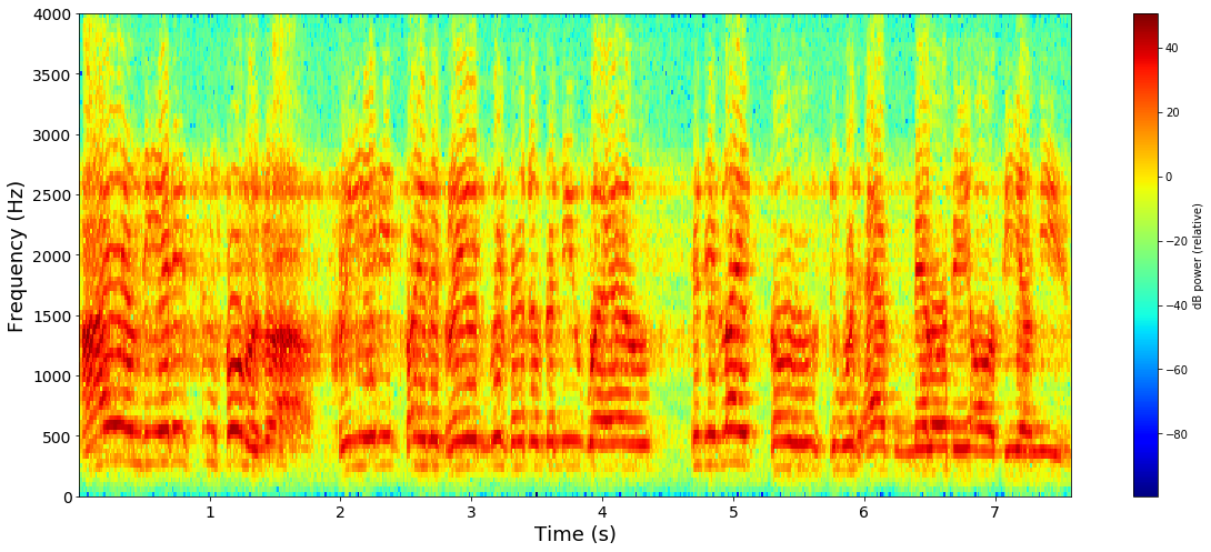
Until the 2010’s, the state-of-the-art for speech recognition models were phonetic-based approaches including separate components for pronunciation, acoustic, and language models. Speech recognition in the past and today both rely on decomposing sound waves into frequency and amplitude using fourier transforms, yielding a spectrogram as shown below.
Training the acoustic model for a traditional speech recognition pipeline that uses Hidden Markov Models (HMM) requires speech+text data, as well as a word to phoneme dictionary. HMMs are generative probabilistic models for sequential data, and are typically evaluated using Levenshtein word error distance, a string metric for measuring differences in strings.
These models can be simplified and made more accurate with speech data that is aligned with phoneme transcriptions, but this a tedious manual task. Because of this effort, phoneme-level transcriptions are less likely to exist for large sets of speech data than word-level transcriptions. For more information on existing open source speech recognition tools and models, check out our colleague Cindi Thompson’s recent post.
Connectionist Temporal Classification (CTC) loss function
We can discard the concept of phonemes when using neural networks for speech recognition by using an objective function that allows for the prediction of character-level transcriptions: Connectionist Temporal Classification (CTC). Briefly, CTC enables the computation of probabilities of multiple sequences, where the sequences are the set of all possible character-level transcriptions of the speech sample. The network uses the objective function to maximize the probability of the character sequence (i.e., chooses the most likely transcription), and calculates the error for the predicted result compared to the actual transcription to update network weights during training.
It is important to note that the character-level error used by a CTC loss function differs from the Levenshtein word error distance often used in traditional speech recognition models. For character generating RNNs, the character and word error distance will be similar in phonetic languages such as Esperonto and Croatian, where individual sounds correspond to distinct characters. Conversely, the character versus word error will be quite different for a non-phonetic language like English.
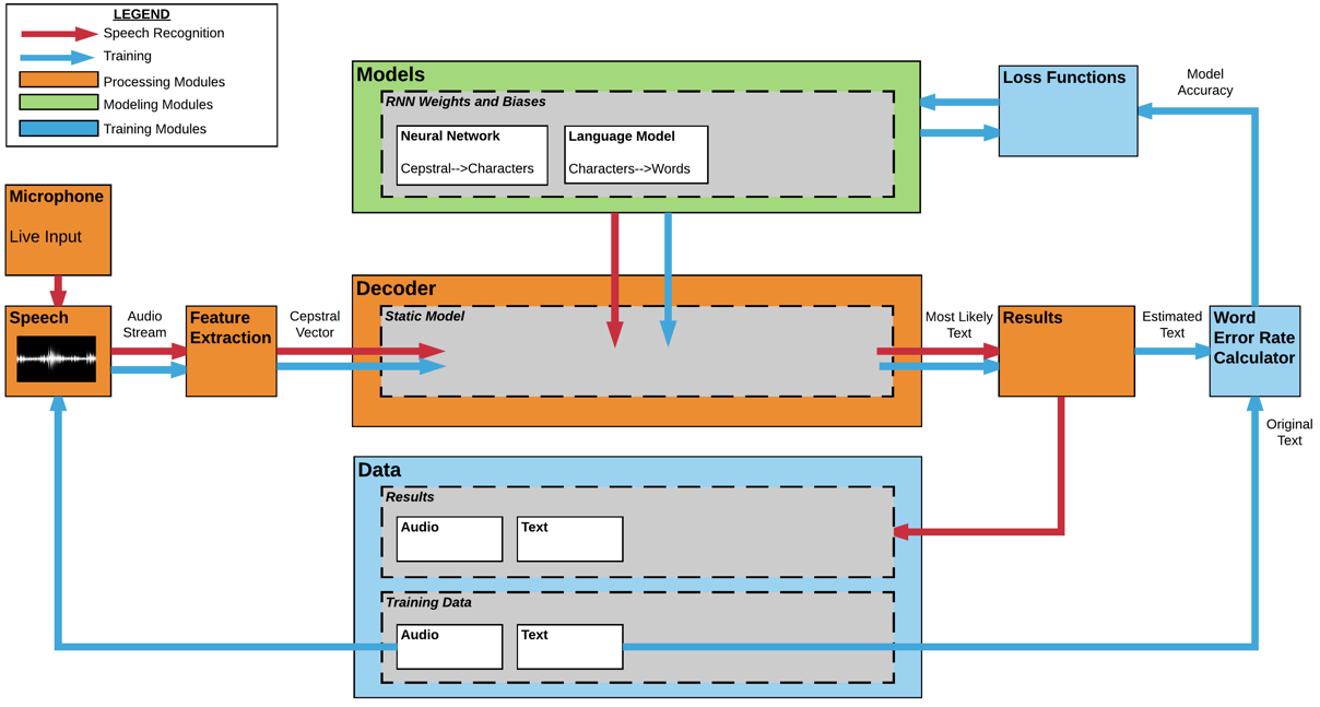
If you want to learn more about CTC, there are many papers and blog posts that explain it in more detail. We will use TensorFlow’s CTC implementation, and there continues to be research and improvements on CTC-related implementations, such as this recent paper from Baidu. In order to utilize algorithms developed for traditional or deep learning speech recognition models, our team structured our speech recognition platform for modularity and fast prototyping:
Importance of data
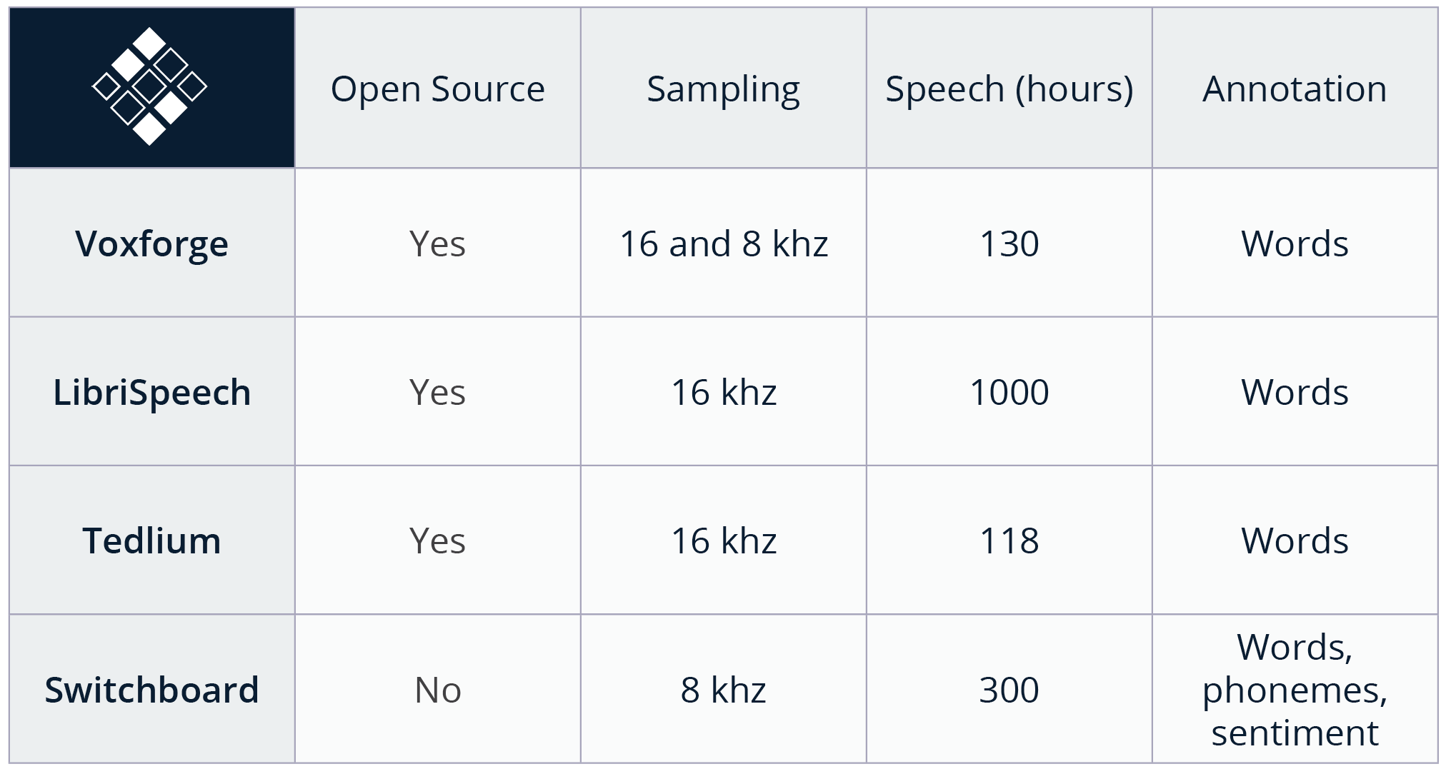
It should be no surprise that creating a system that transforms speech into its textual representation requires having (1) digital audio files and (2) transcriptions of the words that were spoken. Because the model should generalize to decode any new speech samples, the more examples we can train the system on, the better it will perform. We researched freely available recordings of transcribed English speech; some examples that we have used for training are LibriSpeech (1000 hours), TED-LIUM (118 hours), and VoxForge (130 hours). The chart below includes information on these datasets including total size in hours, sampling rate, and annotation.
In order to easily access data from any data source, we store all data in a flat format. This flat format has a single .wav and a single .txt per datum. For example, you can find example Librispeech Training datum ‘211-122425-0059’ in our GitHub repo as 211-122425-0059.wav and 211-122425-0059.txt. These data filenames are loaded into the TensorFlow graph using a datasets object class, that assists TensorFlow in efficiently loading, preprocessing the data, and loading individual batches of data from CPU to GPU memory. An example of the data fields in the datasets object is shown below:
Feature representation
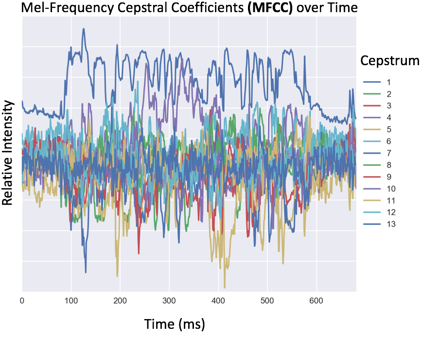
In order for a machine to recognize audio data, the data must first be converted from the time to the frequency domain. There are several methods for creating features for machine learning of audio data, including binning by arbitrary frequencies (i.e., every 100Hz), or by using binning that matches the frequency bands of the human ear. This typical human-centric transformation for speech data is to compute Mel-frequency cepstral coefficients (MFCC), either 13 or 26 different cepstral features, as input for the model. After this transformation the data is stored as a matrix of frequency coefficients (rows) over time (columns).
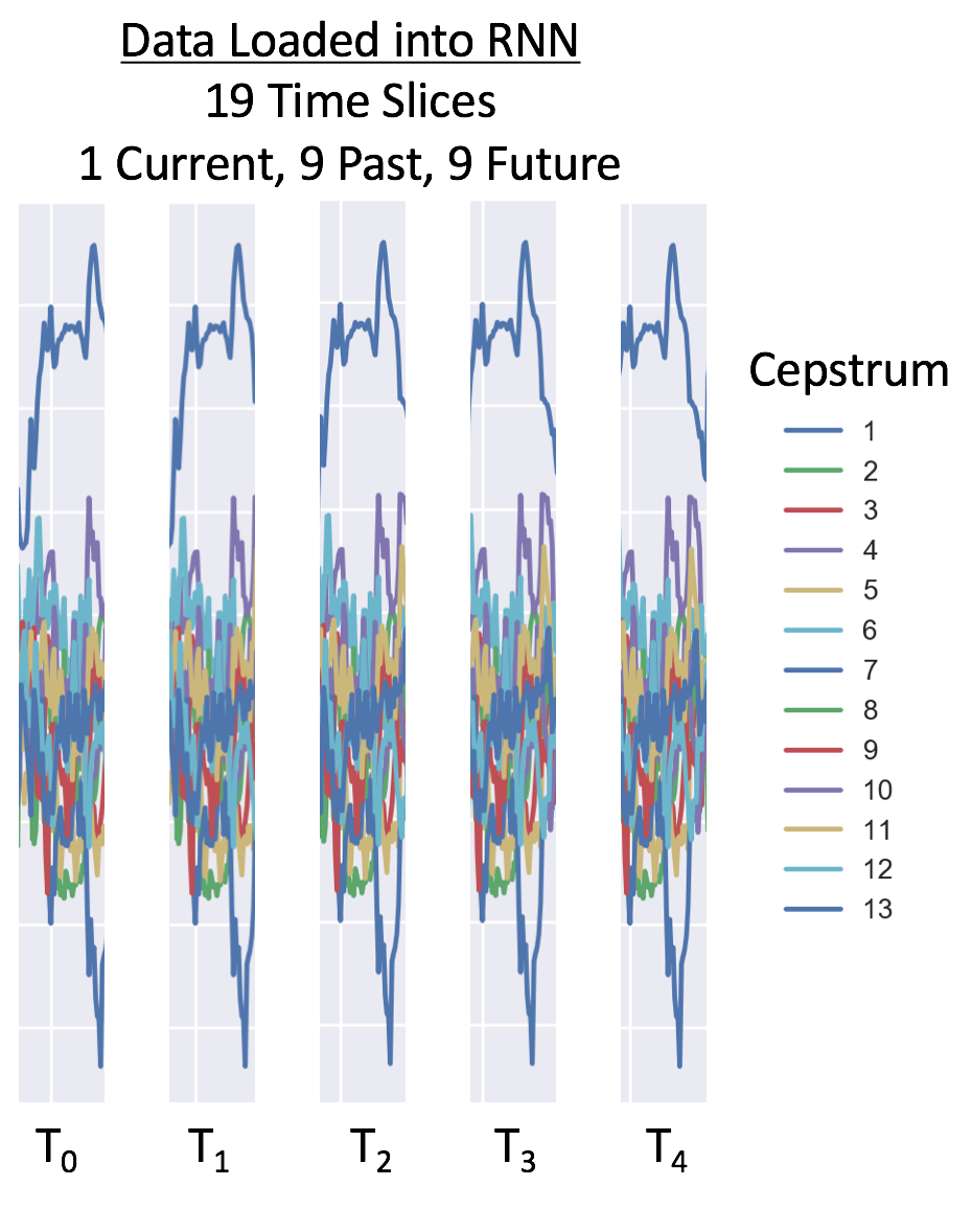
Because speech sounds do not occur in isolation and do not have a one-to-one mapping to characters, we can capture the effects of coarticulation (the articulation of one sound influencing the articulation of another) by training the network on overlapping windows (10s of milliseconds) of audio data that captures sound from before and after the current time index. Example code of how to obtain MFCC features, and how to create windows of audio data is shown below:
For our RNN example, we use 9 time slices before and 9 after, for a total of 19 time points per window.With 26 cepstral coefficients, this is 494 data points per 25 ms observation. Depending on the data sampling rate, we recommend 26 cepstral features for 16,000 Hz and 13 cepstral features for 8,000 hz. Below is an example of data loading windows on 8,000 Hz data:
If you would like to learn more about converting analog to digital sound for RNN speech recognition, check out Adam Geitgey’s machine learning post.
Modeling the sequential nature of speech
Long Short-Term Memory (LSTM) layers are a type of recurrent neural network (RNN) architecture that are useful for modeling data that has long-term sequential dependencies. They are important for time series data because they essentially remember past information at the current time point, which influences their output. This context is useful for speech recognition because of its temporal nature. If you would like to see how LSTM cells are instantiated in TensorFlow, we’ve include example code below from the LSTM layer of our DeepSpeech-inspired Bi-Directional Neural Network (BiRNN).
For more details about this type of network architecture, there are some excellent overviews of how RNNs and LSTM cells work. Additionally, there continues to be research on alternatives to using RNNs for speech recognition, such as with convolutional layers which are more computationally efficient than RNNs.
Network training and monitoring
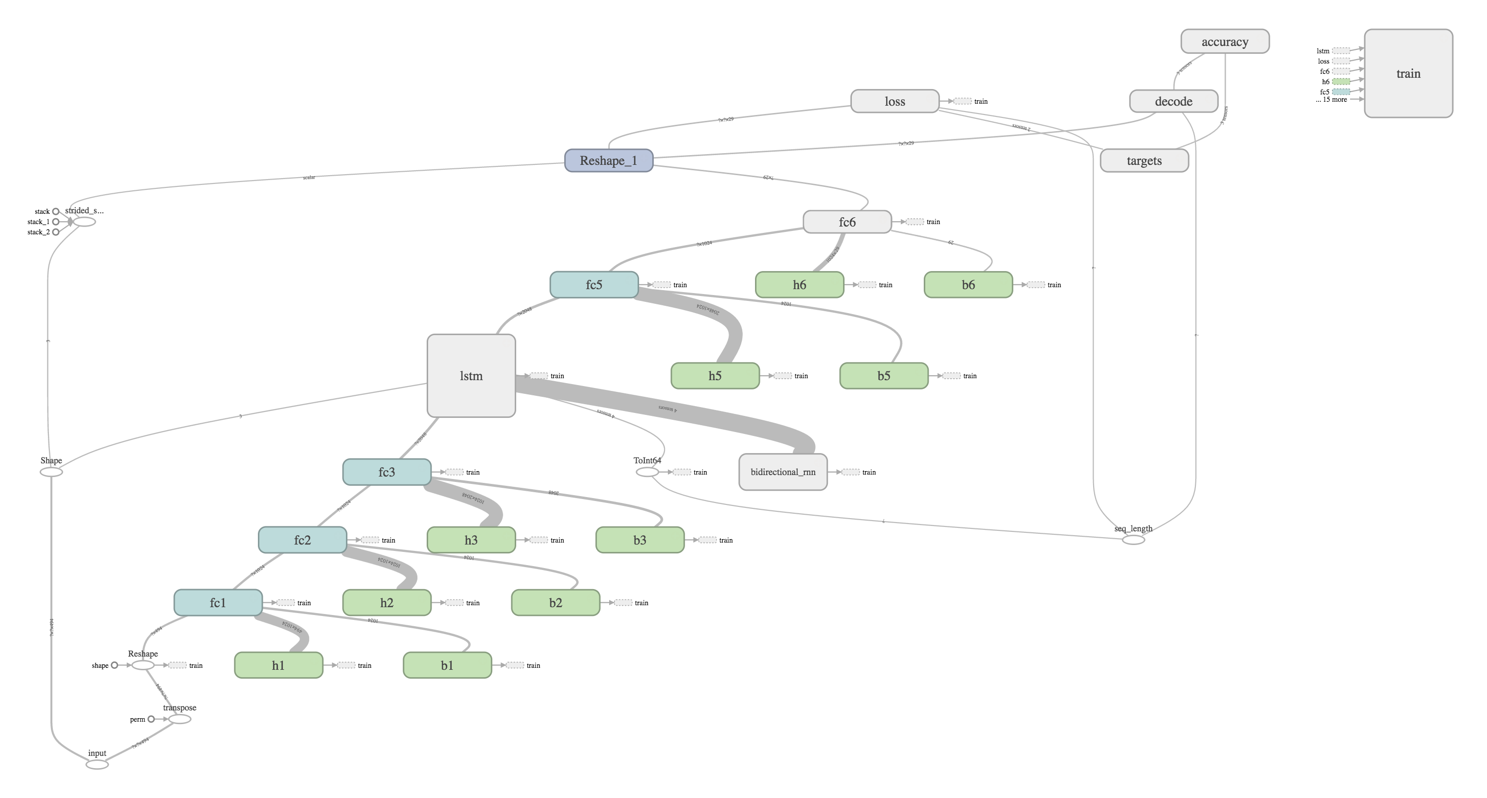
Because we trained our network using TensorFlow, we were able to visualize the computational graph as well as monitor the training, validation, and test performance from a web portal with very little extra effort using TensorBoard. Using tips from Dandelion Mane’s great talk at the 2017TensorFlow Dev Summit, we utilize tf.name_scope to add node and layer names, and write out our summary to file. The results of this is an automatically generated, understandable computational graph, such as this example of a Bi-Directional Neural Network (BiRNN) below. The data is passed amongst different operations from bottom left to top right. The different nodes can be labelled and colored with namespaces for clarity. In this example, teal ‘fc’ boxes correspond to fully connected layers, and the green ‘b’ and ‘h’ boxes correspond to biases and weights, respectively.
We utilized the TensorFlow provided tf.train.AdamOptimizer to control the learning rate. The AdamOptimizer improves on traditional gradient descent by using momentum (moving averages of the parameters), facilitating efficient dynamic adjustment of hyperparameters. We can track the loss and error rate by creating summary scalars of the label error rate:
How to improve an RNN
Now that we have built a simple LSTM RNN network, how do we improve our error rate? Luckily for the open source community, many large companies have published the math that underlies their best performing speech recognition models. In September 2016, Microsoft released a paper in arXiv describing how they achieved a 6.9% error rate on the NIST 200 Switchboard data. They utilized several different acoustic and language models on top of their convolutional+recurrent neural network. Several key improvements that have been made by the Microsoft team and other researchers in the past 4 years include:
- using language models on top of character based RNNs
- using convolutional neural nets (CNNs) for extracting features from the audio
- ensemble models that utilize multiple RNNs
It is important to note that the language models that were pioneered in traditional speech recognition models of the past few decades, are again proving valuable in the deep learning speech recognition models.
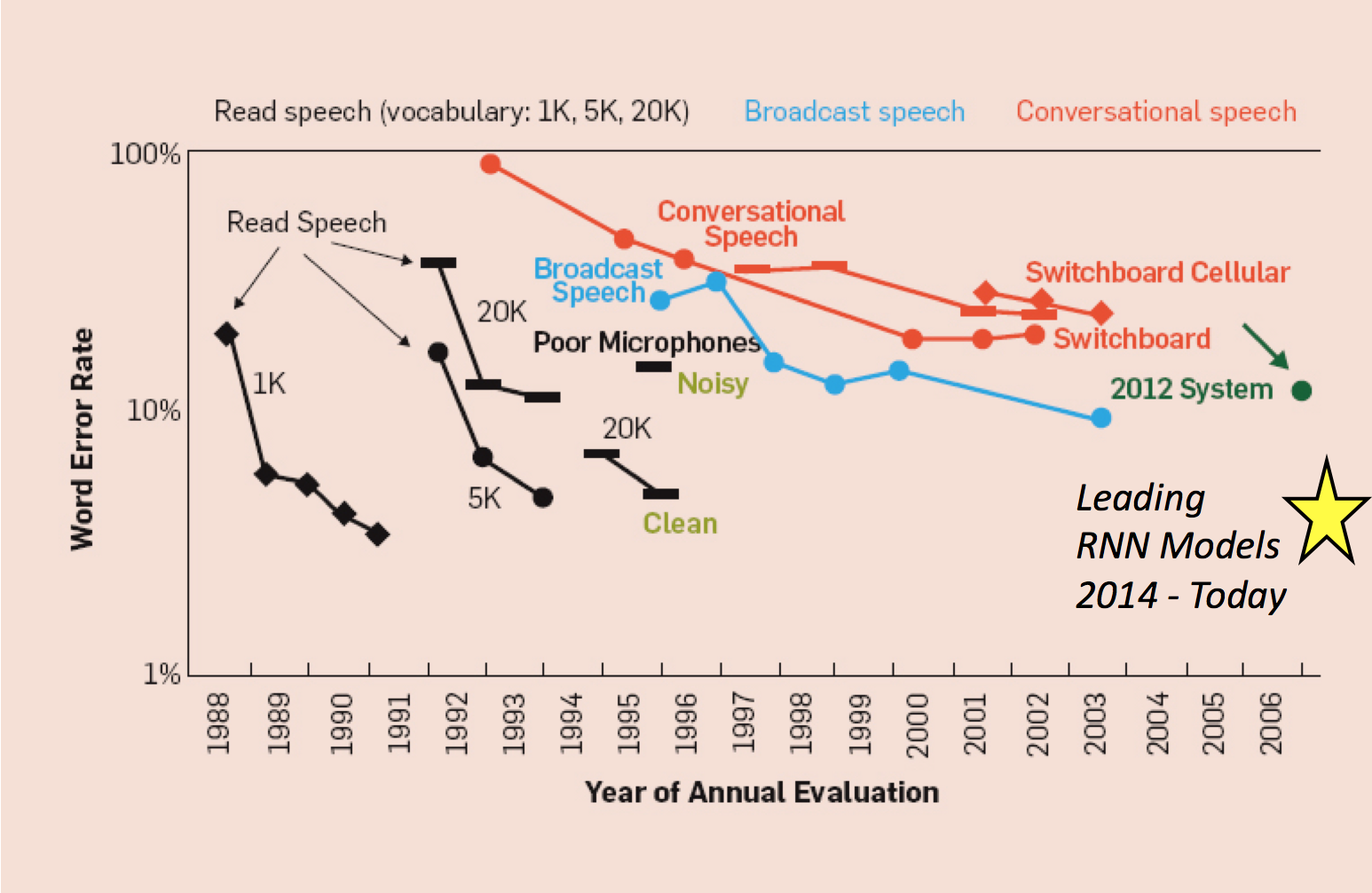
Modified From: A Historical Perspective of Speech Recognition, Xuedong Huang, James Baker, Raj Reddy Communications of the ACM, Vol. 57 No. 1, Pages 94-103, 2014
Training your first RNN
We have provided a GitHub repository with a script that provides a working and straightforward implementation of the steps required to train an end-to-end speech recognition system using RNNs and the CTC loss function in TensorFlow. We have included example data from the LibriVox corpus in the repository. The data is separated into folders:
- Train: train-clean-100-wav (5 examples)
- Test: test-clean-wav (2 examples)
- Dev: dev-clean-wav (2 examples)
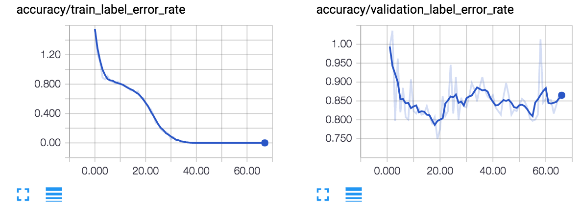
When training these handful of examples, you will quickly notice that the training data will be overfit to ~0% word error rate (WER), while the Test and Dev sets will be at ~85% WER. The reason the test error rate is not 100% is because out of the 29 possible character choices (a-z, apostrophe, space, blank), the network will quickly learn that:
- certain characters (e, a, space, r, s, t) are more common
- consonant-vowel-consonant is a pattern in English
- increased signal amplitude of the MFCC input sound features corresponds to characters a-z
The results of a training run using the default configurations in the github repository is shown below:
If you would like to train a performant model, you can add additional .wav and .txt files to these folders, or create a new folder and update `configs/neural_network.ini` with the folder locations. Note that it can take quite a lot of computational power to process and train on just a few hundred hours of audio, even with a powerful GPU.
We hope that our provided repo is a useful resource for getting started—please share your experiences with adopting RNNs in the comments. To stay in touch, sign up for our newsletter or contact us.
Matthew Rubashkin, with a background in optical physics and biomedical research, has a broad range of experiences in software development, database engineering, and data analytics. He enjoys working closely with clients to develop straightforward and robust solutions to difficult problems.
Matt Mollison, with a background in cognitive psychology and neuroscience, has extensive experience in hypothesis testing and the analysis of complex datasets. He is excited about using predictive models and other statistical methods to solve real-world problems.
Original. Reposted with permission.
Related: