How Feature Engineering Can Help You Do Well in a Kaggle Competition – Part I
As I scroll through the leaderboard page, I found my name in the 19th position, which was the top 2% from nearly 1,000 competitors. Not bad for the first Kaggle competition I had decided to put a real effort in!
By Gabriel Moreira, CI&T.

It is midnight on January 18, 2017, and the Outbrain Click Prediction machine learning competition has just finished. It has been three and a half months of working late. As I scroll through the leaderboard page, I found my name in the 19th position, which was the top 2% from nearly 1,000 competitors. Not bad for the first Kaggle competition I had decided to put a real effort in!

One of the reasons why I managed to score well was the fact that Google Cloud Platform (GCP) made my life easier and I could focus on the data. Now I will take you through my journey!
The challenge
The Kaggle competition was sponsored by Outbrain, which pairs relevant content and readers with 250 billion personalized recommendations every month across several thousand sites. In that competition, ‘Kagglers’ were challenged to predict on which ads and other forms of sponsored content its global base of users would click.
Outbrain maintains a network of publishers and advertisers. In the image below, for example, paid content (ads) are presented to a user in a CNN (publisher) news page.

From Outbrain Click Prediction competition.
In this competition, competitors were asked to accurately rank recommendations by predicted likelihood of being clicked. CTR (Click-Through Rate) prediction is very relevant for industries like e-commerce and advertisement, as tiny improvements in user conversion may lead to significant increases in profits, while providing a better user experience.
Dataset and infrastructure
One of the competition challenges was to handle the massive dataset: 2 billion page views and roughly 17 million click records from 700 million unique users, across 560 sites. It contained a sample of users’ pageviews and clicks, as observed on multiple publishing sites in the United States between June 14, 2016, and June 28, 2016.
Considering it was a large relational database, with some tables not fitting ‘in memory’, Apache Spark was very suitable for data exploration and fast distributed pre-processing. Google Cloud Platform (GCP) provided the main components I needed for storage and distributed processing.
It was easy to deploy a Spark cluster using Google Cloud Dataproc managed service. I found out that a cluster with 1 master and 8 worker nodes of “n1-highmem-4” instance type (~4 CPU cores and 16 GB RAM) was able to process all competition data in about one hour, including joining large tables, transforming features and storing vectors.
My main development environment was Jupyter notebooks, a very productive Python interface. This GCP tutorial describes how to easily set up Jupyter in Dataproc master node, making PySpark libraries available for usage.
Dataproc Spark clusters use Google Cloud Storage (GCS) as distributed file system instead of default HDFS. As a managed storage, it makes it easy to transfer and store large files between instances. Spark jobs are able to use data directly from GCS for distributed processing.
I also employed some machine learning frameworks (FTRL, FFM, GBM, etc.), which worked on parallelized — not distributed — computation, requiring high CPU cores and RAM memory for large datasets. A ‘n1-highmem-32’ instance (32 CPUs and 256 RAM) deployed on Google Compute Engine (GCE) made it possible to run jobs in less than one hour. As their processing was very I/O intensive, I attached a SSD disk to the instance to avoid bottlenecks.
In the second part of this post series, I will talk more about those machine learning models.
First approach
The competition evaluation metric was MAP@12 (Mean Average Precision at 12), which measures the quality of ad ranking. In other words, this metric assesses whether the actual clicked ad was well ranked by the model.
It’s common sense that the ads’ average popularity may be a good predictor of new clicks. The main idea was then to rank ads displayed for users by their decreasing CTR (#clicks / #views).
In the following Python snippets, I show how to compute ads CTR based on train set (click_trains.csv) using PySpark. This CSV file has more than 87 million rows and was stored on GCS. The full script runs in less than 30 seconds in a Dataproc Spark cluster with 8 worker nodes.
In the next snippet, I define a new DataFrame grouping rows by ad_id and aggregating the sum of clicks and count of views. The processing of the CTR is made by a UDF (User Defined Function) named ctr_udf. The snippet output is a table with a sample of 10 ad_ids and their respective #clicks, #views e CTR.
To increase the CTR confidence, we can consider only ads with more than five views. With the collectAsMap() action, the distributed collection is converted to an in-memory lookup dictionary, whose key is the ad_id and the value is the corresponding average CTR.
This was the submitted baseline by most of the competitors and, even without any machine learning algorithm, would give you MAP@12 of 0.637. As a reference, the official baseline competition was based on ads ranking by their ids (random-like approach), for which MAP@12 was 0.485. Thus, this initial approach actually does a nice job for click prediction.
Data Analysis
As always, before applying any machine learning technique, it is very important to analyze the data and to formulate hypotheses about which features and algorithms would be useful to tackle the problem. I implemented an EDA (Exploratory Data Analysis) to unveil the largest dataset (page_views.csv ~ 100 GB) using PySpark.
My EDA Kernel, showing how to use Python, Spark SQL, and Jupyter notebooks in Dataproc to analyze the competition largest dataset, was shared with other competitors and turned out to be the second most-voted contribution (gold medal). Based on my Kernel comments, it appears that many Kagglers are considering trying Google Dataproc and Spark for machine learning competitions.
My analysis helped me to figure out how to extract value from the dataset, by joining it with training and test data (events.csv). For example, in the cumulative chart shown below, we can see that 65% of the users have only one page view, 77%, have at most two views and 89% of the users have at most five views.

Cumulative percentage of users with at most N page views.
This is a typical ‘cold-start’ scenario where we know almost nothing about most users and need to predict which recommended content they will click on.
In general, traditional recommender system techniques like Collaborative Filtering and Content-Based Filtering will fail in this scenario. My strategy was then to employ machine learning algorithms that are able to leverage contextual information about the users’ events and recommended sponsored content.
Feature Engineering
Feature engineering refers to the essential step of selecting or creating the right features to be used in a machine learning model. Usually, it may consume up to 80% of the total effort, depending on the data complexity.
In the following picture, I show the competition original data model, with features colored by their data type.
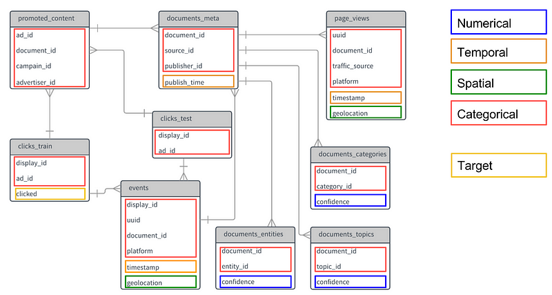
Outbrain Click Prediction large relational database.
All categorical fields were originally represented as integer numbers. Depending on the machine learning algorithm, ids represented as ordinal values may teach the model that one category has a greater relevance than the other. For example, if Argentina id is 1 and Brazil is 2, an algorithm could infer that Brazil is twice as more representative than Argentina. To deal with such issue, it’s common to use techniques like One-Hot Encoding(OHE) where each categorical field is transformed into a sparse vector. In the sparse vector all positions have zero values, except the one corresponding to the id value.
Another popular technique for categorical features with large number of unique values is Feature Hashing, which maps categories to a fixed length vector using hashing functions. This approach provides lower sparsity and higher compression compared to OHE and deals nicely with new and rare categorical values (eg. previously unseen user-agents). It also may cause some collisions when mapping more than one feature to the same vector position, but machine learning algorithms are usually robust enough to deal with these conflicts. I used both techniques in my approach.
I also used ‘Binning’ for the numerical scalar features. Some features are very noisy, and we'd better reduce the effects of minor observation errors or differences with this transformation. For example, I ‘binned’ the event ‘hour’ in periods like morning, midday, afternoon, evening, etc., because my hypotheses is that user behavior wouldn’t be too different if observed at 10am or 11am, for instance.
For long-tail distributed variables, like user_views_count, most users had only one page view logged and very few users with high number of views were present. Applying transformations like log(1 + #views) was useful to smooth out the distribution. A user that has 1,000 page views might not be very different from a user with 500 views, they both are equally outliers in this context.
Standardization and normalization are also important for most machine learning algorithms using optimization techniques like gradient descent. In general, only Decision Trees based models are robust to deal with raw numeric features in different scales and variances.
A more detailed presentation of the main Feature Engineering techniques I have used can be found in this slides.
Based on insights and hypotheses I gleaned from my EDA, I managed to create and transform features for my machine learning models, besides the original features provided in the competition data. Here it follows some of those features.
User profiles
- user_has_already_viewed_doc - For each content recommended to the user, verify whether the user had previously visited that pages.
- user_views_count - Do eager readers behave differently from other users? Let’s add this feature and let machine learning models guess that.
- user_views_categories, user_views_topics, user_views_entities - User profile vectors based on categories, topics and entities of documents that users have previously viewed (weighted by confidence and TF-IDF), to model users preferences in a Content-Based Filtering approach.
- user_avg_views_of_distinct_docs - Ratio between(#user_distinct_docs_views / #user_views), indicating how often users read previously visited pages again.
Ads and Documents
- doc_ad_days_since_published, doc_event_days_since_published - Days elapsed since the ad document was published in a given user visit. The general assumption is that new content is more relevant to users. But if you are reading an old post, you might be interested in other old posts.
- doc_avg_views_by_distinct_users_cf - Average page views of the ad document by distinct users. Is this a webpage people usually return to?
- ad_views_count, doc_views_count - How popular is a document or ad?
Events
- event_local_hour (binned), event_weekend — Event timestamps were in UTC-4, so I processed event geolocation to get timezones and adjust for users' local time. They were binned in periods like morning, afternoon, midday, evening, night. A flag indicating whether it was a weekend was also included. The assumption here is that time influences the kind of content users will read.
- event_country, event_country_state - The field event_geolocation was parsed to extract the user’s country and state in a page visit.
- ad_id, doc_event_id, doc_ad_id, ad_advertiser, … — All of the original categorical fields were One-Hot Encoded to be used by the models, generating about 126,000 features.
Average CTR
- avg_ctr_ad_id, avg_ctr_publisher_id, avg_ctr_advertiser_id, avg_ctr_campain_id, avg_ctr_entity_id_country … - Average CTR (#clicks / #views) given some categorical combinations and CTR confidence (details on Part II post). Eg. P(click | category01, category02).
Content-Based Similarities
These features used TF-IDF technique to build profile vectors for the users and landing pages, modeling user preferences and context respectively. The profiles were compared to candidate ad documents using Cosine Similarity, which is a very popular Information Retrieval based on the angle between of two vectors, ignoring their magnitude.
- user_doc_ad_sim_categories, user_doc_ad_sim_topics, user_doc_ad_sim_entities - Cosine similarity between user profile and ad document profile vectors (TF-IDF).
- doc_event_doc_ad_sim_categories, doc_event_doc_ad_sim_topics, doc_event_doc_ad_sim_entities - Cosine similarity between event document (landing page context) and ad document profile vectors (TF-IDF).
We have generated features based on some of our hypotheses about aspects that might influence users’ decisions on which sponsored content to click on. And the data is now ready for some machine learning models!
Next up…
In the Part II of this post series, I will present the cross-validation strategy, the machine learning models implemented and the ‘Ensemble’ techniques employed to climb up to the Top 2% of the competition leaderboard.
Stay tuned!
Bio: Gabriel Moreira is a scientist passionate about solving problems with data. He is a Doctoral student at Instituto Tecnológico de Aeronáutica - ITA, researching on Recommender Systems and Deep Learning. Currently, he is Lead Data Scientist at CI&T, leading the team in the solution of customer's challenging problems using machine learning on big and unstructured data.
Original. Reposted with permission.
Related: