Train your Deep Learning Faster: FreezeOut
We explain another novel method for much faster training of Deep Learning models by freezing the intermediate layers, and show that it has little or no effect on accuracy.
Deep neural networks have many, many learnable parameters that are used to make inferences. Often, this poses a problem in two ways: Sometimes, the model does not make very accurate predictions. It also takes a long time to train them.
In a previous post, we covered Train your Deep Learning model faster and sharper: Snapshot Ensembling — M models for the cost of 1.
This post talks about reducing training time with little or no impact on accuracy using a novel method.
FreezeOut — Training Acceleration by Progressively Freezing Layers
The authors of this paper propose a method to increase training speed by freezing layers. They experiment with a few different ways of freezing the layers, and demonstrate the training speed up with little(or none) effect on accuracy.
What does Freezing a Layer mean?
Freezing a layer prevents its weights from being modified. This technique is often used in transfer learning, where the base model(trained on some other dataset)is frozen.
How does freezing affect the speed of the model?
If you don’t want to modify the weights of a layer, the backward pass to that layer can be completely avoided, resulting in a significant speed boost. For e.g. if half your model is frozen, and you try to train the model, it will take about half the time compared to a fully trainable model.
On the other hand, you still need to train the model, so if you freeze it too early, it will give inaccurate predictions.
What is the ‘novel’ approach?
The authors demonstrated a way to freeze the layers one by one as soon as possible, resulting in fewer and fewer backward passes, which in turn lowers training time.
At first, the entire model is trainable (exactly like a regular model). After a few iterations the first layer is frozen, and the rest of the model is continued to train. After another few iterations , the next layer is frozen, and so on.
Learning Rate Annealing
The authors used learning rate annealing to govern the learning rate of the model. The notably different technique they used was to change the learning rate layer by layer instead of the whole model. They used the following equation:
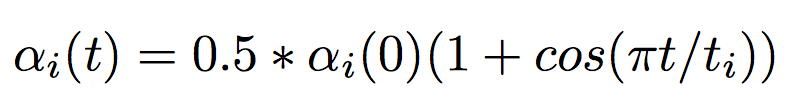
Equation 2.0: α is the learning rate. t is the iteration number. i denotes the ith layer of the model
Equation 2.0 Explanation
The sub i denotes the ith layer. So α sub i denotes the learning rate for the ith layer. Similarly , ti denotes the number of iterations the ith layer has been trained on. t denotes the total number of iterations for the whole model.
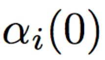
This denotes the initial learning rate for the ith layer.
The authors experimented with different values for Equation 2.1
Initial learning rate for Equation 2.1
The authors tried scaling the initial learning rate so that each layer was trained for an equal amount of time.
Remember that because the first layer of the model would be stopped first, it would be otherwise trained for the least amount of time. To remedy that, they scaled the the learning rate for each layer.
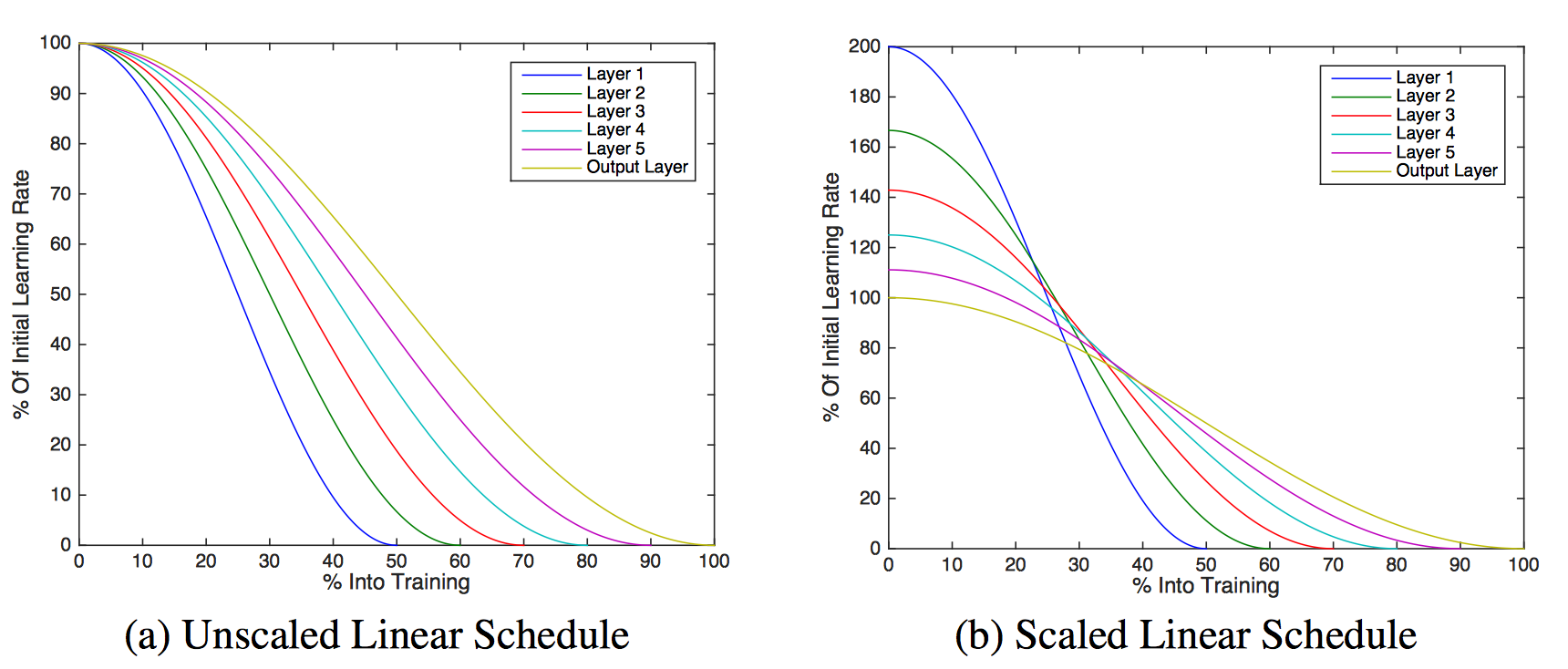
The scaling was done to ensure all the layers’ weights moved equally in the weight space, i.e. the layers that were being trained the longest(the later layers), had a lower learning rate.
The authors also played with cubic scaling, where the value of t sub i is replaced by its own cube.
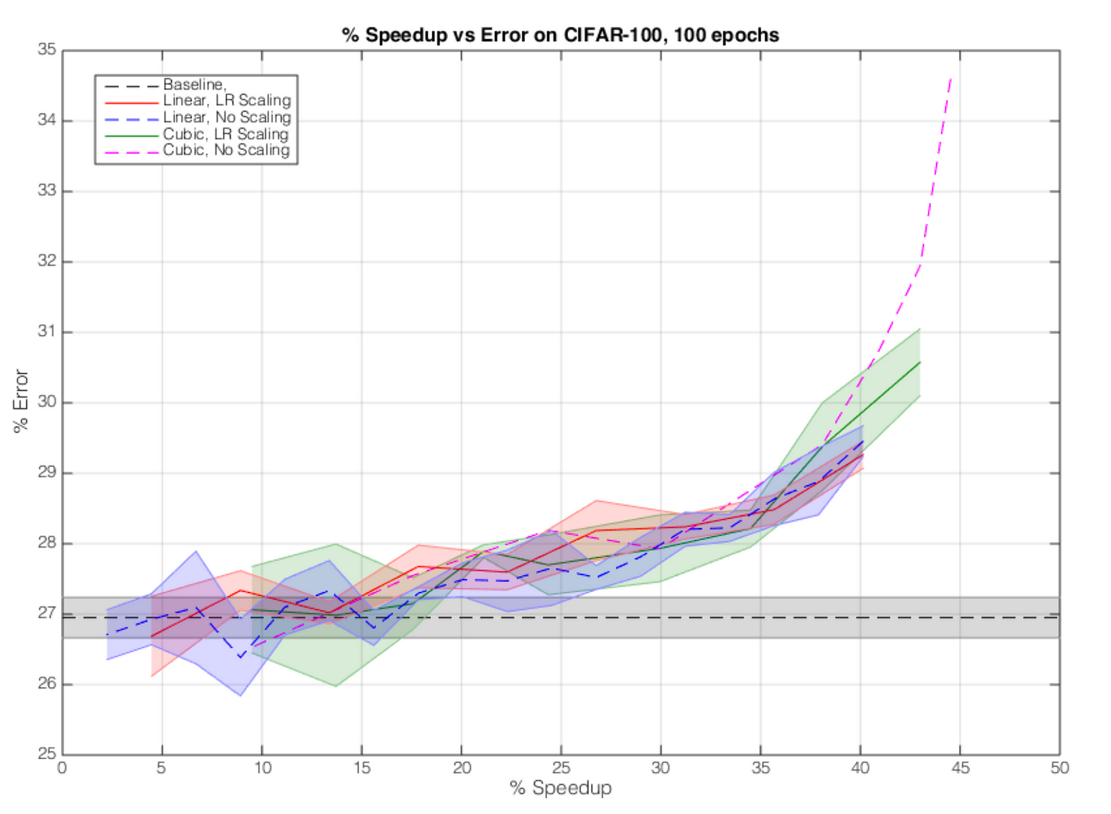
Fig. 2.1: Performance vs Error on DenseNet
The authors have included more benchmarks, and their method increases a training speedup of about 20% at only 3% accuracy drop, and 15% at no drop in accuracy.
Their method does not work very well for models that do not utilize skip connections(such as VGG-16). Neither accuracy not speedups were noticeably different in such networks.
My Bonus Trick
The authors are progressively stopping each layer from being trained, which they then don’t calculate the backward passes for. They seemed to have missed to exploit precomputing layer activations. By doing so, you can even prevent calculating the forward pass.
What is precomputation
This is a trick used in transfer learning. This is the general workflow.
- Freeze the layers you don’t want to modify
- Calculate the activations the last layer from the frozen layers(for your entire dataset)
- Save those activations to disk
- Use those activations as the input of your trainable layers
Since the layers are frozen progressively, the new model can now be seen as a standalone model(a smaller model) , that just takes the input of whatever the last layer outputs. This can be done over and over again as each layer is frozen.
Doing this along with FreezeOut will result in a further substantial reduction in training time while not affecting other metrics(like accuracy) in any way.
Conclusion
I demonstrated 2(and half of my own) very recent and novel techniques to improve accuracy and lower training time by fine tuning learning rates. By also adding pre computation whenever possible, a significant speed boost can be possible using my own proposed method.
Original. Reposted with permission.
Bio: Harshvardhan Gupta writes at HackerNoon.
Related: