Notes on Feature Preprocessing: The What, the Why, and the How

comments

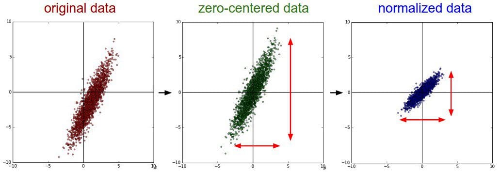
Original vs shifted vs shifted & scaled data (Source: Artificial Intelligence GitBook)

This article covers a few important points related to the preprocessing of numeric data, focusing on the scaling of feature values, and the broad question of dealing with outliers.

Effects of Feature Scaling

 
Feature scaling can be defined as "a method used to standardize the range of independent variables or features of data." Feature scaling is one of the main components of data preprocessing, and can be applied to all types of data one might come across.

Some models are influenced by features scaling, while others are not. Non-tree-based models can be easily influenced by feature scaling:

• Linear models
• Nearest neighbor classifiers
• Neural networks

Conversely, tree-based models are not influenced by feature scaling. It should be obvious, but examples of tree-based modeling algorithms include:

• Plain old decision trees
• Random forests
• Gradient boosted trees

 
Why is this?

Imagine we multiply the scale of a particular feature's values (and only that feature's values) by 100. If we think in terms of the positioning of data points along an axis corresponding to this feature, there will be a clear effect on a model such as a nearest neighbors classifier, for instance. Linear models, nearest neighbors, and neural networks are all sensitive to the relative positioning of data point values to one another; in fact, that's how the explicit premise of K-nearest neighbors (kNN).

Since tree-based models search for the best split positions along a feature's data axis, this relative positioning is far less important. If the determined split position is between points a and b, this will remain constant if both points are multiplied or divided by some constant.

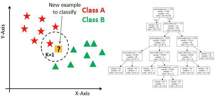
Resulting models from algorithms such as kNN on the left are susceptible to feature scaling; tree-based models such as those on the right are not susceptible to feature scaling

A potential use of feature scaling beyond the obvious is testing feature importance. For kNN, for example, the larger a given feature's values are, the more impact they will have on a model. This fact can be taken advantage of by intentionally boosting the scale of a feature or features which we may believe to be of greater importance, and see if slight deviations in these larger values impact the resulting model. Conversely, multiplying a feature's data point values by zero will result in stacked data points along that axis, rendering this feature useless in the modeling process.

This covers linear models, but what about neural networks? It turns out that neural networks are greatly affected by scale as well: the impact of regularization is proportional to feature scale. Gradient descent methods can have trouble without proper scaling.

Finally, to provide the simplest example of why feature scaling is important: consider k-means clustering. If your data has 4 columns, with 3 of the columns' values being scaled between 0 and 1, and the fourth possessing values between 0 and 1,000, it is relatively easy to determine which of these features will be the sole determinant of clustering results.

Feature Scaling Methods

 
Min/Max Scaling

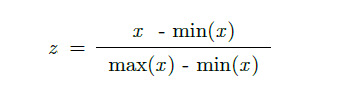
• This method scales values between 0 and 1 ???? [0, 1]
• Sets minimum equal to zero, maximum equal to one, and all other values scaled accordingly in between
• The Scikit-learn sklearn.preprocessing.MinMaxScaler module is such an implementation

from sklearn.preprocessing import MinMaxScaler

# import some data

sc = MinMaxScaler()
data = sc.fit_transform(data))

 
Standard Scaling

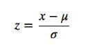
• This method scales by setting the mean of the data to 0, and the standard deviation to 1
• Subtracts the mean value from feature value, and divides by standard deviation
• This results in the standardized distribution
• The Scikit-learn sklearn.preprocessing.StandardScaler module is such an implementation

from sklearn.preprocessing import StandardScaler

# import some data

sc = StandardScaler()
sc.fit_transform(data))

 
What is the difference between these (and other) scaling methods in practice? This is dependent on the specific dataset they are applied to, but in practice the results are often roughly similar.

Dealing with Outliers

 
People often push back hard against talk of "removing outliers." The reality is that outliers can unhelpfully skew a model. The real issue is not that removing outliers is, in itself, an issue; however, you need to understand outliers as they relate to the data, and make an informed judgement as to whether or not they should be removed, and exactly why this is the case. An alternative to removing outliers is using some form of scaling to manage them.

Outliers can be an issue not just for features, but also potentially for target values. If all target values are between 0 and 1, for example, and a new data point is introduced with a target value of 100,000, a resulting regression model would start predicting artificially high values for the rest of our data points in the model.

Keep in mind that outliers can often represent NaNs, especially if they fall outside of upper and lower bounds and are tightly clustered (all NaNs may have been converted to -999, for example). This type of outlier skews distribution artificially, and some approach to dealing with them is absolutely necessary. Domain knowledge and data inspection are the most useful tools for deciding how to deal with outliers.

 
Clipping

One approach to fix outliers for linear models is to keep values between upper and lower bounds. How do we choose these bounds? A reasonable approach is using percentiles -- keep the values between, say, the first and 99th percentiles only. This form of clipping is referred to as winsorization.

Refer to scipy.stats.mstats.winsorize for more info on winsorization.

import numpy as np
from scipy.stats.mstats import winsorize

# import some data

data = winsorize(data, limits = 0.01)

 
Rank Transform

Rank transform removes the relative distance between feature values and replaces them with a consistent interval representing feature value ranking (think: first, second, third...). This moves outliers closer to other feature values (at a regular interval), and can be a valid approach for linear models, kNN, and neural networks.

Refer to scipy.stats.rankdata for more on rank transform.

from scipy.stats import rankdata
rankdata([0, 2, 3, 2])

# Output:
# array([ 1. ,  2.5,  4. ,  2.5])

 
Log Transform

Log transforms can be useful for non-tree-based models. They can be used to drive larger feature values away from extremes and closer to the mean feature values. It also has the effect of making values closer to zero more distinguishable.

See numpy.log and numpy.sqrt for more information on implementing these transforms.

 
It may be useful to combine a variety of preprocessing methods together into one model, by preprocessing percentages of your dataset instances using different methods, and concatenating the results into a single training set. Alternatively, mixing models which were trained on differently preprocessed data (compare with the former method description) via ensembling could also prove useful.

Preprocessing is not a "one size fits all" situation, and your willingness to experiment with alternative approaches based on sound mathematical principles can perhaps lead to increased model robustness.

References:

 
Related:

• 7 Steps to Mastering Data Preparation with Python
• Text Data Preprocessing: A Walkthrough in Python
• Data Preparation Tips, Tricks, and Tools: An Interview with the Insiders