How to count Big Data: Probabilistic data structures and algorithms

Learn how probabilistic data structures and algorithms can be used for cardinality estimation in Big Data streams.

As you might already know, the Big Data is more than simply a matter of size. The datasets of Big Data are larger, more complex, and generated more rapidly than our current resources can handle. Such datasets are so extensive that traditional data processing software and algorithms just can't manage them. This is why Big Data doesn't refer to data, it refers to technology.

The Probabilistic data structures and algorithms (PDSA) are a family of advanced approaches that are optimized to use fixed or sublinear memory and constant execution time; they are often based on hashing and have many other useful features. However, they also have some disadvantages such as they cannot provide the exact answers and have some probability of error (that, actually, can be controlled). The trade-off between the error and the resources is another feature that distinguishes all algorithms and data structures of this family.

Such technologies have found very naturally the use-cases in Big Data, since there we also have the trade-off - either left the whole data unprocessed or agree that some results are not entirely exact.

Just as an example, we can point some algorithms from the PDSA family by addressing The 3 Vs of Big Data.

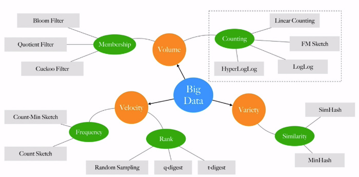
Probabilistic data structures and algorithms are widely used in production already. Everybody knows the simple Bloom Filter, but also there are more sophisticated yet more interesting algorithms as HyperLogLog, q-digest, Count-Min-Sketch, SimHash, and others. PDSA is used in Google BigQuery, Amazon Redshift, Redis, Apache Cassandra, Apache Spark, Elasticsearch, PipelineDB, and others.

If you are interested in learning such algorithms and data structures, please check my recently published book "Probabilistic Data Structures and Algorithms for Big Data Applications" (ISBN: 978-3748190486), where I explain the most popular and widely used algorithms in details.

Counting

In this article, we focus on counting, the task of finding the number of distinct elements in some huge data stream (known as cardinality).

Traditional approach

One of the traditional approaches to counting elements is to build the list of all unique elements we saw thus far. To avoid listing elements twice, we can use store them in a sorted form and search on insert. As soon as we need to answer the query about the number of unique elements , we simply count the number of elements in the list or maintain a separate counter.

The obvious disadvantage of this approach is the linear memory and time complexity, which can be ignored for small datasets but become a problem in Big Data processing.

Let's consider an example. According to the SimilarWeb's traffic overview from June 2019, the Amazon and eBay had about 3.375 billion visitors. If we assume that every 10th of those visitors was unique, we can expect cardinality of such a set at about 337 million and the memory required to store the list of unique elements is 5.4 GB.

But what if I say that we can count them with only about 12KB of memory? Yes, we will lose some exactness, but do we really needed it here?

Here is another example. Katy Perry's Twitter account @katyperry had exactly 107,797,024 followers (as on Jul 30, 2019), but would someone really cry if Twitter just reports about 107M or 108M followers?

I hope you are convinced at this points that there are many practical use-cases where counting error can be tolerated by the efficiency and resources saving.

Probabilistic Counter

We start describing the probabilistic approach to the counting problem with a Probabilistic Counting algorithm that was invented by Philippe Flajolet and G. Nigel Martin in 1985. It is based on hashing and uses the idea of observing common patterns in hashed representations of processing elements.

First of all, every input element is hashed into an integer using some hash function and then that integer is represented as a binary string using LSB-0 notation. For example, assume h("hello") = 42 => "01010100". For every such string, we can compute its "rank", simply the number of leading zeros. Thus, rank("01010100") = 1.

Now the idea is very simple, instead of storing all observed elements, we store only the observed ranks. Since hashing guarantee to compute the same hash for the same input, we can guarantee that we store information only about unique elements. For that, we do not need to allocate huge arrays of integers, because we know the range of the possible values for the rank, which is limited by the length of produced binary strings. Thus, we can store all ranks in a binary array of that length by setting the corresponding bit to one. We can call such a data structure a "Counter" (also known as FM-Sketch). Think, how much memory we have saved comparing the traditional approach above!

We can intuitively expect, that the more values we have seen, the closer we are to the distribution that can be expected theoretically (remind yourself the problem of estimating the number of tails and heads for a coin). And the theoretical expectation is that the probability to observe 1 at some position j in the Counter after indexing n elements is $n/(2^{j+1})$ .

From this formula, we can see that for small indices (low ranks) which $j << log_{2}{n}$ we almost certainly have ones in the Counter. In contrast, for the high ranks that correspond to the big indexes $j >> log_{2}{n}$ we almost certanly will have zeros in the Counter. Only in the range where $j ~ log_{2}{n}$ the probability of seeing one or zero is about to equal.

Thus, to have an idea about the cardinality using such a Counter and assuming that is has indexed "enough" elements, we can use the expectations above. Particularly, we can use the left-most position of zero (R) in the Counters as an indicator of $log_{2}{n}$ and the approximation formula becomes

$n \approx \frac{2^R}{0.77351}$

where $\phi \approx 0.77351$ is a scaling constant.

Thus, using a single binary Counter we can very fast estimate the number of unique elements. The advantage of such an approach comparing to the traditional one is that the memory is fixed regardless of the number of unique elements. However, the weakness of the single-counter approach is that there is a lack of highly confident estimations for the cardinality that means quite a high variance. Thereby, the natural extension of the algorithm is to have simple counters and, consequently, increase the number of estimations. The final prediction can be obtained by averaging the predictions R_k from those counters R_k .

$n \approx \frac{2^{\text{AVG}(R_k)}}{0.77351}$

HyperLogLog

The most popular probabilistic algorithms to estimate cardinality used in practice are from the LogLog family of algorithms that includes the HyperLogLog algorithm, Philippe Flajolet, Éric Fusy, Olivier Gandouet, and Frédéric Meunier in 2007.

Following the generic approach of the Probabilistic Counter, the HyperLogLog algorithm, however, does not stores all observed ranks in Counters but saved only the maximal observed rank for each such a Counter.

To avoid computing different hash functions for each input element , the HyperLogLog uses an approach called stochastic averaging, which allows using only one 32-bit hash function, but reserve some bits from the hash value for addressing (to emulate counters) and use the rest to compute the rank.

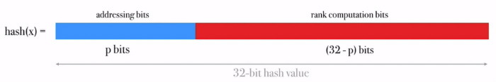
Having addressing bits, we can simulate m=2^p Counters, each of which requires about 4 bytes of memory to store the maximal observed rank.

$n ~ \alpha \dot m * 2^{AVG(R_i)}$

where $\alpha$ is a scaling constant and for some ranges of this formula could be additionally corrected due to bias.

In the video below you can see the HyperLogLog data structure with 64 counters that are populated with about 1K city names from various countries (Note, that not every element updates the counters since we compute only maximal observed values). At the chart below there is how observed relative error in cardinality estimation changes with more elements we index, while at the right you see the current error.

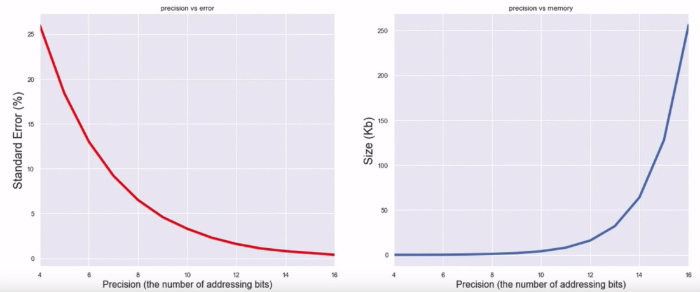
Of course, the more bits we reserve for addressing, the more counters we can simulate. Thus we can expect a smaller error. But the downside is that many counters require more memory. Also, there is a natural limit on addressing bits, since we cannot use more than half of the hash value. Otherwise our rank estimation quality will be hardly affected.

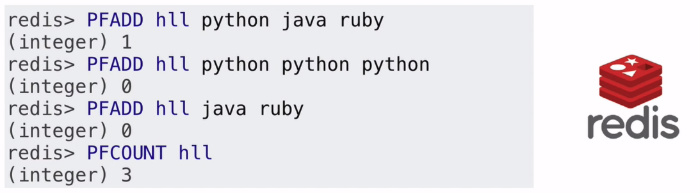
As an example of the application where many of us already use HyperLogLog algorithm is the well-known in-memory database Redis. Its implementation of HyperLogLog requires a small constant amount of memory of 12 KB for every data structure and can approximate the exact cardinality with a standard error of 0.81%.

If you are interested in usage of such data structure from your code, there are plenty of implementation in almost all programming language. I maintain a Python library, PDSA, that is implemented in Cython and can be easily used from any Python applications. By the way, everybody is welcome to contribute!

HyperLogLog++

The article about probabilistic counting will be not complete without an improved version of HyperLogLog, known as HyperLogLog++. It was developed in Google and published by Stefan Heule, Marc Nunkesser, and Alexander Hall in 2013. The improvements are focused on support for even larger cardinalities and better bias correction than in the HyperLogLog algorithm.

The most noticeable improvement of the HyperLogLog++ algorithm is the usage of a 64-bit hash function. Clearly, the longer the output values of the hash function, the more different elements can be encoded. Such improvement allows to estimate cardinalities far larger than 10^9 unique elements, but when the cardinality approaches $2^64 ~ 1.8 \cdot 10^19$ , hash collisions become a problem for the HyperLogLog++ as well.

The algorithm uses exactly the same evaluation function for the number of unique elements but provides better bias correction using pre-trained data. The authors performed a series of experiments to measure the bias and found that some extreme cases the bias of the original HyperLogLog algorithm could be further corrected using empirical data collected over the experiments.

Additionally, the HyperLogLog++ algorithm proposed a sparse version of storing internal counters, but it is out of the scope for this very brief article.

Conclusion

In this article, we learned about probabilistic data structures and algorithms and studied how we can use them in such a complex task as cardinality estimation for Big Data streams. If you are interested in more information about the material covered here or want to read the original papers, please take a look at the list of references that follows this article.

Resources

Probabilistic Data Structures and Algorithms for Big Data Applications book
Probabilistic Counting Algorithms for Data Base Applications article by Philippe Flajolet and G. Nigel Martin
Hyperloglog: The analysis of a near-optimal cardinality estimation algorithm article by Philippe Flajolet et al.
Redis new data structure: the HyperLogLog blog post by @antirez
HyperLogLog in Practice article by Stefan Heule et al.

Bio: Andrii Gakhov (@gakhov) is a mathematician and software engineer holding a Ph.D. in mathematical modeling and numerical methods. He has been a teacher in the School of Computer Science at V. Karazin Kharkiv National University in Ukraine for a number of years and currently works as a software practitioner for ferret go GmbH, the leading community moderation, automation, and analytics company in Germany.

Related:

How to count Big Data: Probabilistic data structures and algorithms

Counting

Conclusion

More On This Topic

Latest Posts

Top Posts