Data Science 101: Preventing Overfitting in Neural Networks

One method of combating overfitting is called regularization. Regularization modifies the objective function that we minimize by adding additional terms that penalize large weights. In other words, we change the objective function so that it becomes Error+λf(θ), where f(θ) grows larger as the components of θ grow larger and λ is the regularization strength (a hyper-parameter for the learning algorithm). The value we choose for λ determines how much we want to protect against overfitting. A λ=0 implies that we do not take any measures against the possibility of overfitting. If λ is too large, then our model will prioritize keeping θ as small as possible over trying to find the parameter values that perform well on our training set. As a result, choosing λ is a very important task and can require some trial and error.

The most common type of regularization is L2 regularization. It can be implemented by augmenting the error function with the squared magnitude of all weights in the neural network. In other words, for every weight w in the neural network, we add 1/2 λw^2 to the error function. The L2 regularization has the intuitive interpretation of heavily penalizing "peaky" weight vectors and preferring diffuse weight vectors. This has the appealing property of encouraging the network to use all of its inputs a little rather than using only some of its inputs a lot. Of particular note is that during the gradient descent update, using the L2 regularization ultimately means that every weight is decayed linearly to zero. Because of this phenomenon, L2 regularization is also commonly referred to as weight decay.

We can visualize the effects of L2 regularization using ConvnetJs. Similar to above, we use a neural network with two inputs, a soft-max output of size two, and a hidden layer with 20 neurons. We train the networks using mini-batch gradient descent (batch size 10) and regularization strengths of 0.01, 0.1, and 1. The results can be seen below.

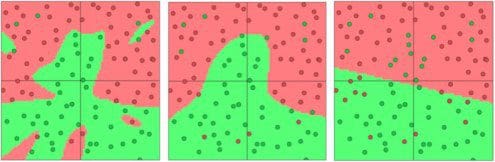
Fig 5. Separating green dots vs red dots, L2 regularization strengths of 0.01, 0.1, and 1

Another common type of regularization is L1 regularization. Here, we add the term λ|w| for every weight win the neural network. The L1 regularization has the intriguing property that it leads the weight vectors to become sparse during optimization (i.e. very close to exactly zero). In other words, neurons with L1 regularization end up using only a small subset of their most important inputs and become quite resistant to noise in the inputs.

In comparison, weight vectors from L2 regularization are usually diffuse, small numbers. L1 regularization is very useful when you want to understand exactly which features are contributing to a decision. If this level of feature analysis isn't necessary, we prefer to use L2 regularization because it empirically performs better.

Max norm constraints have a similar goal of attempting to restrict from θ becoming too large, but they do this more directly. Max norm constraints enforce an absolute upper bound on the magnitude of the incoming weight vector for every neuron and use projected gradient descent to enforce the constraint. In other words, anytime a gradient descent step moved the incoming weight vector such that ||w||₂ >c, we project the vector back onto the ball (centered at the origin) with radius c. One of the nice properties is that the parameter vector cannot grow out of control (even if the learning rates are too high) because the updates to the weights are always bounded.

Dropout is a very different kind of method for preventing overfitting that can often be used in lieu of other techniques. While training, dropout is implemented by only keeping a neuron active with some probability p (a hyperparameter), or setting it to zero otherwise. Intuitively, this forces the network to be accurate even in the absence of certain information. It prevents the network from becoming too dependent on any one (or any small combination) of neurons. Expressed more mathematically, it prevents overfitting by providing a way of approximately combining exponentially many different neural network architectures efficiently. The process of dropout is expressed pictorially in the figure below.

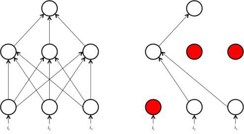
Fig 6. Drop-out in Neural networks

In this article, we’ve discussed the problem of overfitting and its exacerbation in deep neural networks. We’ve also gone over a number of techniques to prevent overfitting from happening during the training process, including regularization, max norm constraints, and dropout. These techniques are critical in deep learning because they enable us to properly sufficiently complex models even when our datasets are relatively limited. Overfitting protection is an area of very active research, so if you have any cool ideas about how to tackle this challenging problem, please feel free to drop me a line at nkbuduma@gmail.com!

Bio: Nikhil Buduma is a computer science student at MIT with deep interests in machine learning and the biomedical sciences. He is a two time gold medalist at the International Biology Olympiad, a student researcher, and a “hacker.”

• Inside Deep Learning: Computer Vision With Convolutional Neural Networks
• Deep Learning, The Curse of Dimensionality, and Autoencoders
• Deep Learning in a Nutshell – what it is, how it works, why care?