Must Know Tips for Deep Learning Neural Networks

Now the data is ready. However, before you are beginning to train the network, you have to initialize its parameters.

All Zero Initialization

In the ideal situation, with proper data normalization it is reasonable to assume that approximately half of the weights will be positive and half of them will be negative. A reasonable-sounding idea then might be to set all the initial weights to zero, which you expect to be the “best guess” in expectation. But, this turns out to be a mistake, because if every neuron in the network computes the same output, then they will also all compute the same gradients during back-propagation and undergo the exact same parameter updates. In other words, there is no source of asymmetry between neurons if their weights are initialized to be the same.

Initialization with Small Random Numbers

Thus, you still want the weights to be very close to zero, but not identically zero. In this way, you can random these neurons to small numbers which are very close to zero, and it is treated as symmetry breaking. The idea is that the neurons are all random and unique in the beginning, so they will compute distinct updates and integrate themselves as diverse parts of the full network. The implementation for weights might simply look like weights ~ 0.001 × N(0,1), where N(0,1) is a zero mean, unit standard deviation gaussian. It is also possible to use small numbers drawn from a uniform distribution, but this seems to have relatively little impact on the final performance in practice.

Calibrating the Variances

One problem with the above suggestion is that the distribution of the outputs from a randomly initialized neuron has a variance that grows with the number of inputs. It turns out that you can normalize the variance of each neuron's output to 1 by scaling its weight vector by the square root of its fan-in (i.e., its number of inputs), which is as follows:

>>> w = np.random.randn(n) / sqrt(n) # calibrating the variances with 1/sqrt(n)

where “randn” is the aforementioned Gaussian and “n” is the number of its inputs. This ensures that all neurons in the network initially have approximately the same output distribution and empirically improves the rate of convergence. The detailed derivations can be found from Page. 18 to 23 of the slides. Please note that, in the derivations, it does not consider the influence of ReLU neurons.

Current Recommendation

As aforementioned, the previous initialization by calibrating the variances of neurons is without considering ReLUs. A more recent paper on this topic by He et al. [4] derives an initialization specifically for ReLUs, reaching the conclusion that the variance of neurons in the network should be 2.0/n as:

>>> w = np.random.randn(n) * sqrt(2.0/n) # current recommendation

which is the current recommendation for use in practice, as discussed in [4].

Now, everything is ready. Let’s start to train deep networks!

Filters and pooling size. During training, the size of input images prefers to be power-of-2, such as 32 (e.g., CIFAR-10), 64, 224 (e.g., common used ImageNet), 384 or 512, etc. Moreover, it is important to employ a small filter (e.g., 3 × 3) and small strides (e.g., 1) with zeros-padding, which not only reduces the number of parameters, but improves the accuracy rates of the whole deep network. Meanwhile, a special case mentioned above, i.e., 3 × 3 filters with stride 1, could preserve the spatial size of images/feature maps. For the pooling layers, the common used pooling size is of 2 × 2.

Learning rate. In addition, as described in a blog by Ilya Sutskever [2], he recommended to divide the gradients by mini batch size. Thus, you should not always change the learning rates (LR), if you change the mini batch size. For obtaining an appropriate LR, utilizing the validation set is an effective way. Usually, a typical value of LR in the beginning of your training is 0.1. In practice, if you see that you stopped making progress on the validation set, divide the LR by 2 (or by 5), and keep going, which might give you a surprise.

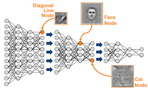
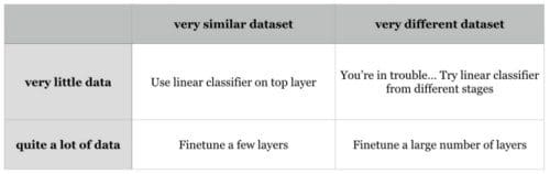
Fine-tune on pre-trained models. Nowadays, many state-of-the-arts deep networks are released by famous research groups, i.e., Caffe Model Zoo and VGG Group. Thanks to the wonderful generalization abilities of pre-trained deep models, you could employ these pre-trained models for your own applications directly. For further improving the classification performance on your data set, a very simple yet effective approach is to fine-tune the pre-trained models on your own data. As shown in following table, the two most important factors are the size of the new data set (small or big), and its similarity to the original data set. Different strategies of fine-tuning can be utilized in different situations. For instance, a good case is that your new data set is very similar to the data used for training pre-trained models. In that case, if you have very little data, you can just train a linear classifier on the features extracted from the top layers of pre-trained models. If your have quite a lot of data at hand, please fine-tune a few top layers of pre-trained models with a small learning rate. However, if your own data set is quite different from the data used in pre-trained models but with enough training images, a large number of layers should be fine-tuned on your data also with a small learning rate for improving performance. However, if your data set not only contains little data, but is very different from the data used in pre-trained models, you will be in trouble. Since the data is limited, it seems better to only train a linear classifier. Since the data set is very different, it might not be best to train the classifier from the top of the network, which contains more dataset-specific features. Instead, it might work better to train the SVM classifier on activations/features from somewhere earlier in the network.

Fine-tune your data on pre-trained models. Different strategies of fine-tuning are utilized in different situations. For data sets, Caltech-101 is similar to ImageNet, where both two are object-centric image data sets; while Place Database is different from ImageNet, where one is scene-centric and the other is object-centric.

Editor's note: Join us tomorrow for the remaining 4 tips & tricks of this fascinating post.

Bio: Xiu-Shen Wei is a 2nd-year Ph.D. candidate of Department of Computer Science and Technology in Nanjing University and a member of LAMDA Group.

Original. Reposted with permission.

Related:

• What To Expect from Deep Learning in 2016 and Beyond
• 7 Steps to Understanding Deep Learning
• Is Deep Learning Overhyped?