Would You Survive the Titanic? A Guide to Machine Learning in Python Part 2
This is part 2 of a 3 part introductory series on machine learning in Python, using the Titanic dataset.
Classification - The Fun Part
We will start off with a simple decision tree classifier. A decision tree examines one variable at a time, and splits into one of two branches based on the result of that value, at which point it does the same for the next variable. A fantasic visual explanation of how decision trees work can be found here.
This is what a trained decision tree for the Titanic dataset looks like, if we set the maximum number of levels to 3:
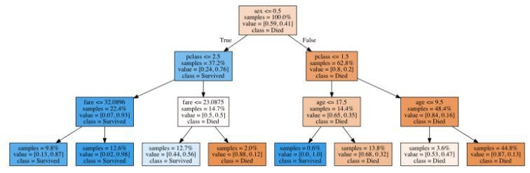
The tree first splits by sex, and then by class, since it has learned during the training phase that these are the two most important features for determining survival. The dark blue boxes indicate passengers who are likely to survive, and the dark orange boxes represent passengers who are almost certainly doomed. Interestingly, after splitting by class, the main deciding factor determining the survival of women is the ticket fare that they paid, while the deciding factor for men is their age(with children being much more likely to survive).
To create this tree, first we initialize an instance of an untrained decision tree classifier(here we will set the maximum depth of the tree to 10). Next we “fit” this classifier to our training set, enabling it to learn about how different factors affect the survivability of a passenger. Now that the decision tree is ready, we can “score” it using our test data to determine how accurate it is.
clf_dt = tree.DecisionTreeClassifier(max_depth=10)

clf_dt.fit (X_train, y_train)
clf_dt.score (X_test, y_test)

# 0.78947368421052633
The resulting reading, 0.7703, means that the model correctly predicted the survival of 77% of the test set. Not bad for our first model!
If you are being an attentive, skeptical reader(as you should be), you might be thinking that the accuracy of the model could vary somewhat depending on which rows were selected for the training and test sets. We will get around this problem by using a shuffle validator.
shuffle_validator = cross_validation.ShuffleSplit(len(X), n_iter=20, test_size=0.2, random_state=0)
def test_classifier(clf):
    scores = cross_validation.cross_val_score(clf, X, y, cv=shuffle_validator)
    print("Accuracy: %0.4f (+/- %0.2f)" % (scores.mean(), scores.std()))

test_classifier(clf_dt)

# Accuracy: 0.7742 (+/- 0.02)
This shuffle validator applies the same random 20:80 split as before, but this time generates 20 unique permutations of this split. By passing this shuffle validator as a parameter to the “cross_val_score” function, we can score our classifier against each of the different splits, and compute the average accuracy and standard deviation from the results.
The result shows that our decision tree classifier has an overall accuracy of 77.34%, although it can go up to 80% and down to 75% depending on the training/test split. Using scikit-learn, we can easily test other machine learning algorithms using the exact same syntax.
clf_rf = ske.RandomForestClassifier(n_estimators=50)
test_classifier(clf_rf)

# Accuracy: 0.7837 (+/- 0.02)

clf_gb = ske.GradientBoostingClassifier(n_estimators=50)
test_classifier(clf_gb)

# Accuracy: 0.8201 (+/- 0.02)

eclf = ske.VotingClassifier([('dt', clf_dt), ('rf', clf_rf), ('gb', clf_gb)])
test_classifier(eclf)

# Accuracy: 0.8036 (+/- 0.02)
The “Random Forest” classification algorithm will create a multitude of (generally very poor) trees for the dataset using different random subsets of the input variables, and will return whichever prediction was returned by the most trees. This helps to avoid “overfitting”, a problem that occurs when a model is so tightly fitted to arbitrary correlations in the training data that it performs poorly on test data.
The “Gradient Boosting” classifier will generate many weak, shallow prediction trees, and will combine, or “boost”, them into a strong model. This model performs very well on our dataset, but has the drawback of being relatively slow and difficult to optimize, as the model construction happens sequentially so cannot be parallelized.
A “Voting” classifier can be used to apply multiple conceptually divergent classification models to the same dataset, and will return the majority vote from all of the classifiers. For instance, if the gradient boosting classifier predicts that a passenger will not survive, but the decision tree and random forest classifiers predict that they will live, the voting classifier will chose the later.
This has been a very brief and non-technical overview of each technique, so I encourage you to learn more about the mathematical implementations of all of these algorithms to obtain a deeper understanding of their relative strengths and weaknesses. Many more classification algorithms are available “out-of-the-box” in scikit-learn and can be explored here.
 Bio: Patrick Triest is a 23 year old Android Developer / IoT Engineer / Data Scientist / wannabe pioneer, originally from Boston and now working at SocialCops. He’s addicted to learning, and sometimes after figuring out something particularly cool he gets really excited and writes about it.
Original. Reposted with permission.
Related: