A Beginner’s Guide To Understanding Convolutional Neural Networks Part 2

This is the second part of a thorough introductory treatment of convolutional neural networks. Have a look after reading the first part.

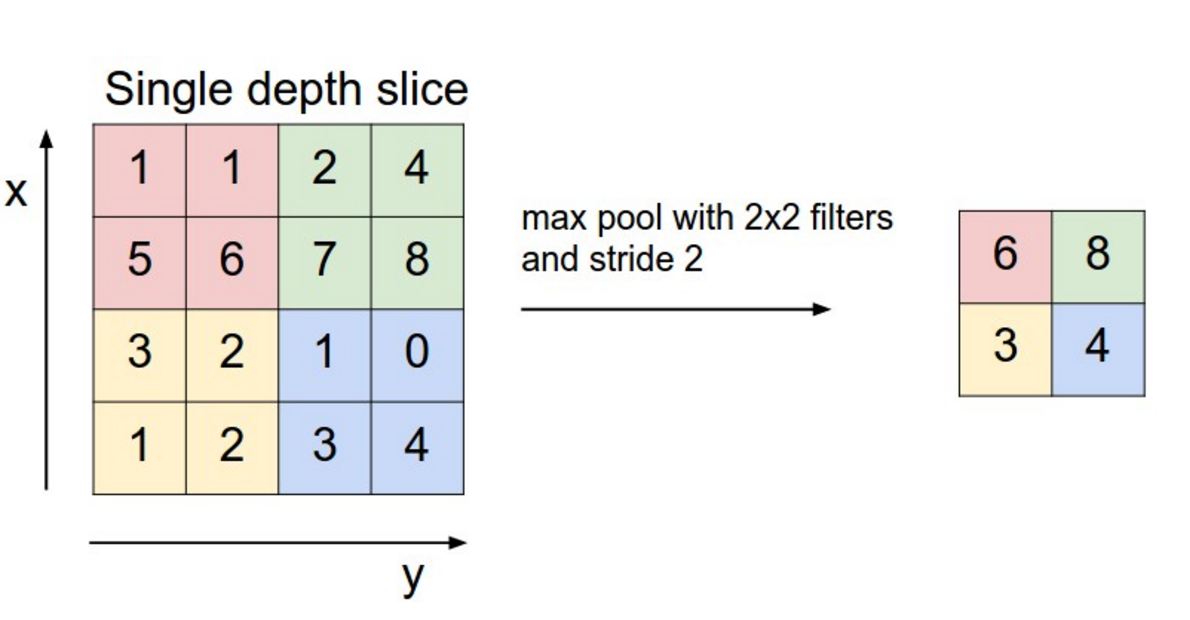
By Adit Deshpande, UCLA on September 8, 2016 in Beginners, Convolutional Neural Networks, Deep Learning, Neural Networks

Pooling Layers

After some ReLU layers, programmers may choose to apply a pooling layer. It is also referred to as a downsampling layer. In this category, there are also several layer options, with maxpooling being the most popular. This basically takes a filter (normally of size 2x2) and a stride of the same length. It then applies it to the input volume and outputs the maximum number in every subregion that the filter convolves around.

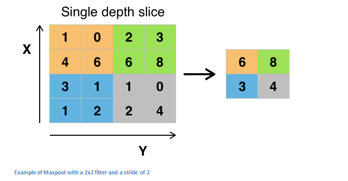
Other options for pooling layers are average pooling and L2-norm pooling. The intuitive reasoning behind this layer is that once we know that a specific feature is in the original input volume (there will be a high activation value), its exact location is not as important as its relative location to the other features. As you can imagine, this layer drastically reduces the spatial dimension (the length and the width change but not the depth) of the input volume. This serves two main purposes. The first is that the amount of parameters or weights is reduced by 75%, thus lessening the computation cost. The second is that it will controloverfitting. This term refers to when a model is so tuned to the training examples that it is not able to generalize well for the validation and test sets. A symptom of overfitting is having a model that gets 100% or 99% on the training set, but only 50% on the test data.

Dropout Layers

Now, dropout layers have a very specific function in neural networks. In the last section, we discussed the problem of overfitting, where after training, the weights of the network are so tuned to the training examples they are given that the network doesn’t perform well when given new examples. The idea of dropout is simplistic in nature. This layer “drops out” a random set of activations in that layer by setting them to zero in the forward pass. Simple as that. Now, what are the benefits of such a simple and seemingly unnecessary and counterintuitive process? Well, in a way, it forces the network to be redundant. By that I mean the network should be able to provide the right classification or output for a specific example even if some of the activations are dropped out. It makes sure that the network isn’t getting too “fitted” to the training data and thus helps alleviate the overfitting problem. An important note is that this layer is only used during training, and not during test time.

Paper by Geoffrey Hinton.

Network in Network Layers

A network in network layer refers to a conv layer where a 1 x 1 size filter is used. Now, at first look, you might wonder why this type of layer would even be helpful since receptive fields are normally larger than the space they map to. However, we must remember that these 1x1 convolutions span a certain depth, so we can think of it as a 1 x 1 x N convolution where N is the number of filters applied in the layer. Effectively, this layer is performing a N-D element-wise multiplication where N is the depth of the input volume into the layer.

Paper by Min Lin.

Classification, Localization, Detection, Segmentation

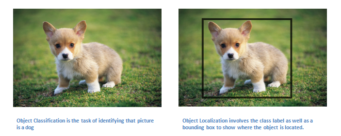
In the example we used in Part 1 of this series, we looked at the task of image classification. This is the process of taking an input image and outputting a class number out of a set of categories. However, when we take a task like object localization, our job is not only to produce a class label but also a bounding box that describes where the object is in the picture.

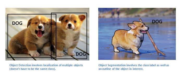
We also have the task of object detection, where localization needs to be done on all of the objects in the image. Therefore, you will have multiple bounding boxes and multiple class labels.

Finally, we also have object segmentation where the task is to output a class label as well as an outline of every object in the input image.

More detail on how these are implemented to come in Part 3, but for those who can’t wait...

Detection/ Localization: RCNN, Fast RCNN, Faster RCNN, MultiBox, Bayesian Optimization, Multi-region, RCNN Minus R, Image Windows
Segmentation: Semantic Seg, Unconstrained Video, Shape Guided, Object Regions, Shape Sharing

Yeah, there’s a lot more.

Transfer Learning

Now, a common misconception in the DL community is that without a Google-esque amount of data, you can’t possibly hope to create effective deep learning models. While data is a critical part of creating the network, the idea of transfer learning has helped to lessen the data demands. Transfer learning is the process of taking a pre-trained model (the weights and parameters of a network that has been trained on a large dataset by somebody else) and “fine-tuning” the model with your own dataset. The idea is that this pre-trained model will act as a feature extractor. You will remove the last layer of the network and replace it with your own classifier (depending on what your problem space is). You then freeze the weights of all the other layers and train the network normally (Freezing the layers means not changing the weights during gradient descent/optimization).

Let’s investigate why this works. Let’s say the pre-trained model that we’re talking about was trained on ImageNet (For those that aren’t familiar, ImageNet is a dataset that contains 14 million images with over 1,000 classes). When we think about the lower layers of the network, we know that they will detect features like edges and curves. Now, unless you have a very unique problem space and dataset, your network is going to need to detect curves and edges as well. Rather than training the whole network through a random initialization of weights, we can use the weights of the pre-trained model (and freeze them) and focus on the more important layers (ones that are higher up) for training. If your dataset is quite different than something like ImageNet, then you’d want to train more of your layers and freeze only a couple of the low layers.

Paper by Yoshua Bengio (another deep learning pioneer).
Paper by Ali Sharif Razavian.
Paper by Jeff Donahue.

Data Augmentation Techniques

By now, we’re all probably numb to the importance of data in ConvNets, so let’s talk about ways that you can make your existing dataset even larger, just with a couple easy transformations. Like we’ve mentioned before, when a computer takes an image as an input, it will take in an array of pixel values. Let’s say that the whole image is shifted left by 1 pixel. To you and me, this change is imperceptible. However, to a computer, this shift can be fairly significant as the classification or label of the image doesn’t change, while the array does. Approaches that alter the training data in ways that change the array representation while keeping the label the same are known as data augmentation techniques. They are a way to artificially expand your dataset. Some popular augmentations people use are grayscales, horizontal flips, vertical flips, random crops, color jitters, translations, rotations, and much more. By applying just a couple of these transformations to your training data, you can easily double or triple the number of training examples.

Sources:

Bio: Adit Deshpande is currently a second year undergraduate student majoring in computer science and minoring in Bioinformatics at UCLA. He is passionate about applying his knowledge of machine learning and computer vision to areas in healthcare where better solutions can be engineered for doctors and patients.

Original. Reposted with permission.

Related: