A Quick Introduction to Neural Networks

The Multi Layer Perceptron shown in Figure 5 (adapted from Sebastian Raschka's excellent visual explanation of the backpropagation algorithm) has two nodes in the input layer (apart from the Bias node) which take the inputs 'Hours Studied' and 'Mid Term Marks'. It also has a hidden layer with two nodes (apart from the Bias node). The output layer has two nodes as well - the upper node outputs the probability of 'Pass' while the lower node outputs the probability of 'Fail'.

In classification tasks, we generally use a Softmax function as the Activation Function in the Output layer of the Multi Layer Perceptron to ensure that the outputs are probabilities and they add up to 1. The Softmax function takes a vector of arbitrary real-valued scores and squashes it to a vector of values between zero and one that sum to one. So, in this case,

Probability (Pass) + Probability (Fail) = 1

Step 1: Forward Propagation

All weights in the network are randomly assigned. Lets consider the hidden layer node marked V in Figure 5 below. Assume the weights of the connections from the inputs to that node are w1, w2 and w3 (as shown).

The network then takes the first training example as input (we know that for inputs 35 and 67, the probability of Pass is 1).

• Input to the network = [35, 67]
• Desired output from the network (target) = [1, 0]

Then output V from the node in consideration can be calculated as below (f is an activation function such as sigmoid):

V = f (1*w1 + 35*w2 + 67*w3)

Similarly, outputs from the other node in the hidden layer is also calculated. The outputs of the two nodes in the hidden layer act as inputs to the two nodes in the output layer. This enables us to calculate output probabilities from the two nodes in output layer.

Suppose the output probabilities from the two nodes in the output layer are 0.4 and 0.6 respectively (since the weights are randomly assigned, outputs will also be random). We can see that the calculated probabilities (0.4 and 0.6) are very far from the desired probabilities (1 and 0 respectively), hence the network in Figure 5 is said to have an 'Incorrect Output'.

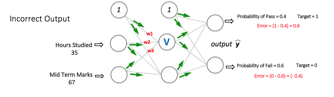
Figure 5: forward propagation step in a multi layer perceptron

Step 2: Back Propagation and Weight Updating

We calculate the total error at the output nodes and propagate these errors back through the network using Backpropagation to calculate the gradients. Then we use an optimization method such as Gradient Descent to 'adjust' all weights in the network with an aim of reducing the error at the output layer. This is shown in the Figure 6 below (ignore the mathematical equations in the figure for now).

Suppose that the new weights associated with the node in consideration are w4, w5 and w6 (after Backpropagation and adjusting weights).

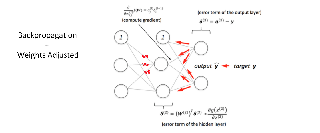
Figure 6: backward propagation and weight updation step in a multi layer perceptron

If we now input the same example to the network again, the network should perform better than before since the weights have now been adjusted to minimize the error in prediction. As shown in Figure 7, the errors at the output nodes now reduce to [0.2, -0.2] as compared to [0.6, -0.4] earlier. This means that our network has learned to correctly classify our first training example.

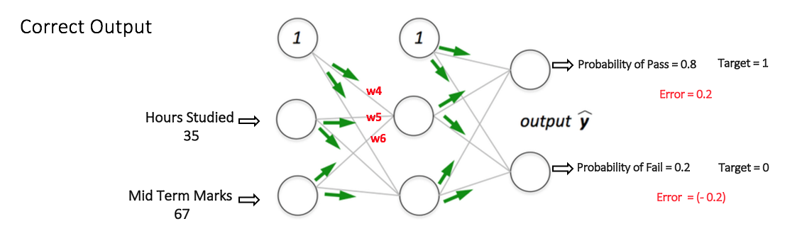
Figure 7: the MLP network now performs better on the same input

We repeat this process with all other training examples in our dataset. Then, our network is said to have learned those examples.

If we now want to predict whether a student studying 25 hours and having 70 marks in the mid term will pass the final term, we go through the forward propagation step and find the output probabilities for Pass and Fail.

I have avoided mathematical equations and explanation of concepts such as 'Gradient Descent' here and have rather tried to develop an intuition for the algorithm. For a more mathematically involved discussion of the Backpropagation algorithm, refer to this link.

3d Visualization of a Multi Layer Perceptron

Adam Harley has created a 3d visualization of a Multi Layer Perceptron which has already been trained (using Backpropagation) on the MNIST Database of handwritten digits.

The network takes 784 numeric pixel values as inputs from a 28 x 28 image of a handwritten digit (it has 784 nodes in the Input Layer corresponding to pixels). The network has 300 nodes in the first hidden layer, 100 nodes in the second hidden layer, and 10 nodes in the output layer (corresponding to the 10 digits) [15].

Although the network described here is much larger (uses more hidden layers and nodes) compared to the one we discussed in the previous section, all computations in the forward propagation step and backpropagation step are done in the same way (at each node) as discussed before.

Figure 8 shows the network when the input is the digit '5'.

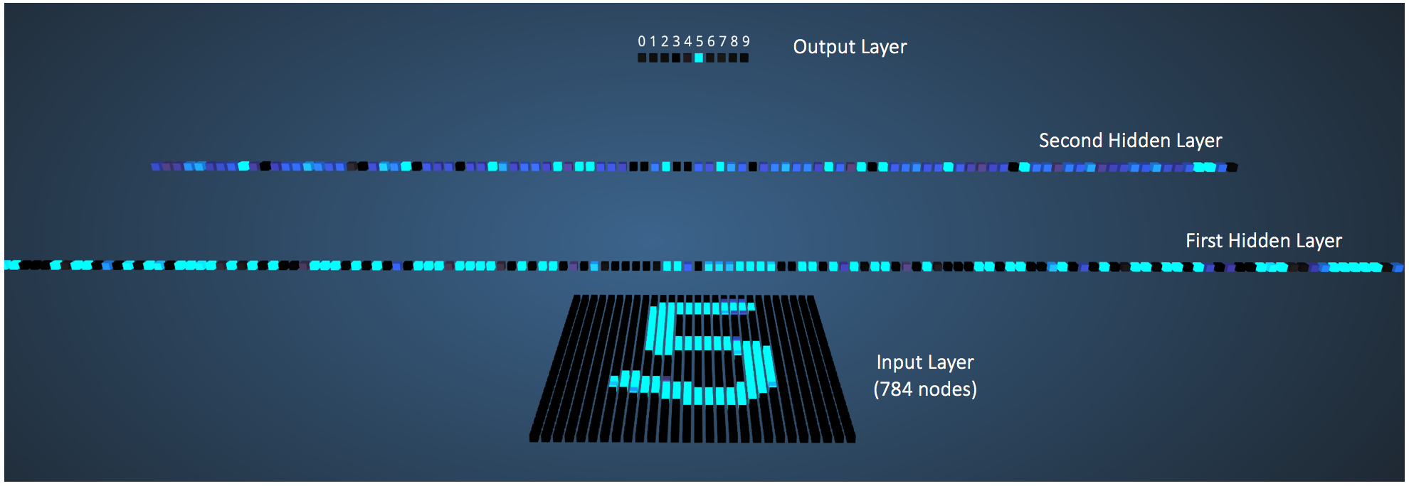
Figure 8: visualizing the network for an input of '5'

A node which has a higher output value than others is represented by a brighter color. In the Input layer, the bright nodes are those which receive higher numerical pixel values as input. Notice how in the output layer, the only bright node corresponds to the digit 5 (it has an output probability of 1, which is higher than the other nine nodes which have an output probability of 0). This indicates that the MLP has correctly classified the input digit. I highly recommend playing around with this visualization and observing connections between nodes of different layers.

Deep Neural Networks

1. What is the difference between deep learning and usual machine learning?
2. What is the difference between a neural network and a deep neural network?
3. How is deep learning different from multilayer perceptron?

Conclusion

I have skipped important details of some of the concepts discussed in this post to facilitate understanding. I would recommend going through Part1, Part2, Part3 and Case Study from Stanford's Neural Network tutorial for a thorough understanding of Multi Layer Perceptrons.

Let me know in the comments below if you have any questions or suggestions!

Bio: Ujjwal Karn has 3 years of industry and research experience in machine learning and is interested in practical applications of deep learning to language and vision understanding.

References

1. Artificial Neuron Models
2. Neural Networks Part 1: Setting up the Architecture (Stanford CNN Tutorial)
3. Wikipedia article on Feed Forward Neural Network
4. Wikipedia article on Perceptron
5. Single-layer Neural Networks (Perceptrons)
6. Single Layer Perceptrons
7. Weighted Networks – The Perceptron
8. Neural network models (supervised) (scikit learn documentation)
9. What does the hidden layer in a neural network compute?
10. How to choose the number of hidden layers and nodes in a feedforward neural network?
11. Crash Introduction to Artificial Neural Networks
12. Why the BIAS is necessary in ANN? Should we have separate BIAS for each layer?
13. Basic Neural Network Tutorial – Theory
14. Neural Networks Demystified (Video Series): Part 1, Welch Labs @ MLconf SF
15. A. W. Harley, "An Interactive Node-Link Visualization of Convolutional Neural Networks," in ISVC, pages 867-877, 2015 (link)

Original.