17 More Must-Know Data Science Interview Questions and Answers

Q4. Why might it be preferable to include fewer predictors over many?

Anmol Rajpurohit answers:

Here are a few reasons why it might be a better idea to have fewer predictor variables rather than having many of them:

Redundancy/Irrelevance:

If you are dealing with many predictor variables, then the chances are high that there are hidden relationships between some of them, leading to redundancy. Unless you identify and handle this redundancy (by selecting only the non-redundant predictor variables) in the early phase of data analysis, it can be a huge drag on your succeeding steps.

It is also likely that not all predictor variables are having a considerable impact on the dependent variable(s). You should make sure that the set of predictor variables you select to work on does not have any irrelevant ones – even if you know that data model will take care of them by giving them lower significance.

Note: Redundancy and Irrelevance are two different notions –a relevant feature can be redundant due to the presence of other relevant feature(s).

Overfitting:

Even when you have a large number of predictor variables with no relationships between any of them, it would still be preferred to work with fewer predictors. The data models with large number of predictors (also referred to as complex models) often suffer from the problem of overfitting, in which case the data model performs great on training data, but performs poorly on test data.

Productivity:

Let’s say you have a project where there are a large number of predictors and all of them are relevant (i.e. have measurable impact on the dependent variable). So, you would obviously want to work with all of them in order to have a data model with very high success rate. While this approach may sound very enticing, practical considerations (such of amount of data available, storage and compute resources, time taken for completion, etc.) make it nearly impossible.

Thus, even when you have a large number of relevant predictor variables, it is a good idea to work with fewer predictors (shortlisted through feature selection or developed through feature extraction). This is essentially similar to the Pareto principle, which states that for many events, roughly 80% of the effects come from 20% of the causes.

Focusing on those 20% most significant predictor variables will be of great help in building data models with considerable success rate in a reasonable time, without needing non-practical amount of data or other resources.

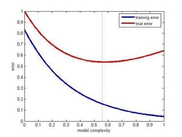
Training error & test error vs model complexity (Source: Posted on Quora by Sergul Aydore)

Understandability:

Models with fewer predictors are way easier to understand and explain. As the data science steps will be performed by humans and the results will be presented (and hopefully, used) by humans, it is important to consider the comprehensive ability of human brain. This is basically a trade-off – you are letting go of some potential benefits to your data model’s success rate, while simultaneously making your data model easier to understand and optimize.

This factor is particularly important if at the end of your project you need to present your results to someone, who is interested in not just high success rate, but also in understanding what is happening “under the hood”.

Q5. What error metric would you use to evaluate how good a binary classifier is? What if the classes are imbalanced? What if there are more than 2 groups?

Prasad Pore answers:

Binary classification involves classifying the data into two groups, e.g. whether or not a customer buys a particular product or not (Yes/No), based on independent variables such as gender, age, location etc.

As the target variable is not continuous, binary classification model predicts the probability of a target variable to be Yes/No. To evaluate such a model, a metric called the confusion matrix is used, also called the classification or co-incidence matrix. With the help of a confusion matrix, we can calculate important performance measures:

1. True Positive Rate (TPR) or Hit Rate or Recall or Sensitivity = TP / (TP + FN)
2. False Positive Rate(FPR) or False Alarm Rate = 1 - Specificity = 1 - (TN / (TN + FP))
3. Accuracy = (TP + TN) / (TP + TN + FP + FN)
4. Error Rate = 1 – accuracy or (FP + FN) / (TP + TN + FP + FN)
5. Precision = TP / (TP + FP)
6. F-measure: 2 / ( (1 / Precision) + (1 / Recall) )
7. ROC (Receiver Operating Characteristics) = plot of FPR vs TPR
8. AUC (Area Under the Curve)
9. Kappa statistics

You can find more details about these measures here: The Best Metric to Measure Accuracy of Classification Models.

All of these measures should be used with domain skills and balanced, as, for example, if you only get a higher TPR in predicting patients who don’t have cancer, it will not help at all in diagnosing cancer.

In the same example of cancer diagnosis data, if only 2% or less of the patients have cancer, then this would be a case of class imbalance, as the percentage of cancer patients is very small compared to rest of the population. There are main 2 approaches to handle this issue:

1. Use of a cost function: In this approach, a cost associated with misclassifying data is evaluated with the help of a cost matrix (similar to the confusion matrix, but more concerned with False Positives and False Negatives). The main aim is to reduce the cost of misclassifying. The cost of a False Negative is always more than the cost of a False Positive. e.g. wrongly predicting a cancer patient to be cancer-free is more dangerous than wrongly predicting a cancer-free patient to have cancer.

Total Cost = Cost of FN * Count of FN + Cost of FP * Count of FP

2. Use of different sampling methods: In this approach, you can use over-sampling, under-sampling, or hybrid sampling. In over-sampling, minority class observations are replicated to balance the data. Replication of observations leading to overfitting, causing good accuracy in training but less accuracy in unseen data. In under-sampling, the majority class observations are removed causing loss of information. It is helpful in reducing processing time and storage, but only useful if you have a large data set.

Find more about class imbalance here.

If there are multiple classes in the target variable, then a confusion matrix of dimensions equal to the number of classes is formed, and all performance measures can be calculated for each of the classes. This is called a multiclass confusion matrix. e.g. there are 3 classes X, Y, Z in the response variable, so recall for each class will be calculated as below:

Recall_X = TP_X/(TP_X+FN_X)

Recall_Y = TP_Y/(TP_Y+FN_Y)

Recall_Z = TP_Z/(TP_Z+FN_Z)

Q6. What are some ways I can make my model more robust to outliers?

Thuy Pham answers:

There are several ways to make a model more robust to outliers, from different points of view (data preparation or model building). An outlier in the question and answer is assumed being unwanted, unexpected, or a must-be-wrong value to the human’s knowledge so far (e.g. no one is 200 years old) rather than a rare event which is possible but rare.

Outliers are usually defined in relation to the distribution. Thus outliers could be removed in the pre-processing step (before any learning step), by using standard deviations (for normality) or interquartile ranges (for not normal/unknown) as threshold levels.

Outliers. Image source

Moreover, data transformation (e.g. log transformation) may help if data have a noticeable tail. When outliers related to the sensitivity of the collecting instrument which may not precisely record small values, Winsorization may be useful. This type of transformation (named after Charles P. Winsor (1895–1951)) has the same effect as clipping signals (i.e. replaces extreme data values with less extreme values).  Another option to reduce the influence of outliers is using mean absolute difference rather mean squared error.

For model building, some models are resistant to outliers (e.g. tree-based approaches) or non-parametric tests. Similar to the median effect, tree models divide each node into two in each split. Thus, at each split, all data points in a bucket could be equally treated regardless of extreme values they may have. The study [Pham 2016] proposed a detection model that incorporates interquartile information of data to predict outliers of the data.

References:

[Pham 2016] T. T. Pham, C. Thamrin, P. D. Robinson, and P. H. W. Leong. Respiratory artefact removal in forced oscillation measurements: A machine learning approach. IEEE Transactions on Biomedical Engineering, 2016.

This Quora answer contains further information.

Here is part 2 and part 3 with more answers.