How To Write Better SQL Queries: The Definitive Guide – Part 2

Time Complexity & The Big O

 
Now that you have examined the query plan briefly, you can start digging deeper and think about the performance in more formal terms with the help of the computational complexity theory. This area in theoretical computer science that focuses on classifying computational problems according to their difficulty, among other things; These computational problems can be algorithms, but also queries.

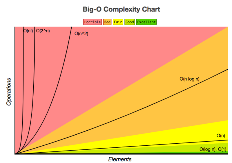
For queries, however, you’re not necessarily classifying them according to their difficulty, but rather to the time it takes to run it and get some results back. This specifically is referred to as time complexity and to articulate or measure this type of complexity, you can use the big O notation.

With the big O notation, you express the runtime in terms of how quickly it grows relative to the input, as the input gets arbitrarily large. The big O notation excludes coefficients and lower order terms so that you can focus on the important part of your query’s running time: its rate of growth. When expressed this way, dropping coefficients and lower order terms, the time complexity is said to be described asymptotically. That means that the input size goes to infinity.

In database language, the complexity measures how much longer it takes a query to run as the size of the data tables, and therefore the database, increase.

Note that the size of your database doesn’t only increase as more data is stored in tables, but also the mere fact that indexes are present in the database also plays a role in the size.

Estimating Time Complexity of Your Query Plan

 
As you have seen before, the execution plan defines, among other things, what algorithm is used for each operation, which makes that every query execution time can be logically expressed as a function of the table size involved in the query plan, which is referred to as a complexity function. In other words, you can use the big O notation and your execution plan to estimate the query complexity and the performance.

In the following subsections, you’ll get a general idea about the four types of time complexities and you’ll see some examples of how queries’ time complexity can vary according to the context in which you run it.

Hint: the indexes are part of the story here!

Note, though, that there are different types of indexes, different execution plans and different implementations for different databases to consider, so that the time complexities listed below are very general and can vary according to your specific setting.

O(1): Constant Time

 
An algorithm is said to run in constant time if it requires the same amount of time regardless of the input size. When you’re talking about a query, it will run in constant time if it requires the same amount of time regardless of the table size.

These type of queries are not really common, yet here’s one such an example:

SELECT TOP 1 t.* 
FROM t

The time complexity is constant because you select one arbitrary row from the table. Therefore, the length of the time should be independent of the size of the table.

Linear Time: O(n)

 
An algorithm is said to run in linear time if its time execution is directly proportional to the input size, i.e. time grows linearly as input size increases. For databases, this means that the time execution would be directly proportional to the table size: as the number of rows in the table grows, the time for the query grows.

An example is a query with a WHERE clause on a un-indexed column: a full table scan or Seq Scan will be needed, which will result in a time complexity of O(n). This means that every row needs to be read to find the one with the right ID. You don’t have a limit at all, so every row does need to be read, even if the first row matches the condition.

Consider also the following example of a query that would have a complexity of O(n) if there’s no index on i_id:

SELECT i_id 
FROM item;

• The previous also means that other queries, such as count queries like COUNT(*) FROM TABLE; will have a time complexity of O(n), because a full table scan will be required unless the total row count is stored for the table. Then, the complexity would be more like O(1).

Closely related to the linear execution time is the execution time for execution plans that have joins in them. Here are some examples:

• A hash join has an expected complexity O(M + N). The classic hash join algorithm for an inner join of two tables first prepares a hash table of the smaller table. The hash table entries consist of the join attribute and its row. The hash table is accessed by applying a hash function to the join attribute. Once the hash table is built, the larger table is scanned and the relevant rows from the smaller table are found by looking in the hash table.
• Merge joins generally have a complexity of O(M+N) but it will heavily depend on the indexes on the join columns and, in cases where there is no index, on whether the rows are sorted according to the keys used in the join:
  • If both tables that are sorted according to the keys that are being used in the join, then the query will have a time complexity of O(M+N).
  • If both tables have an index on the joined columns, then the index already maintains those columns in order and there’s no need to sort. The complexity will be O(M + N).
  • If neither table has an index on the joined columns, a sort of both tables will need to happen first, so the complexity will look more like O(M log M + N log N).
  • If only one of the tables has an index on the joined columns, only the one table that doesn’t have the index will need to be sorted before the merge step can happen, so the complexity will look like O(M + N log N).
• For nested joins, the complexity is generally O(MN). This join is efficient when one or both of the tables are extremely small (for example, smaller than 10 records), which is a very common situation when evaluating queries because some subqueries are written to return only one row.

Remember: a nested join is a join that compares every record in one table against every record in the other.

Logarithmic Time: O(log (n))

 
An algorithm is said to run in logarithmic time if its time execution is proportional to the logarithm of the input size; For queries, this means that they will run if the execution time is proportional to the logarithm of the database size.

This logarithmic time complexity is true for query plans where an Index Scan or clustered index scan is performed. A clustered index is an index where the leaf level of the index contains the actual data rows of the table. A clustered is much like any other index: it is defined on one or more columns. These form the index key. The clustering key is then the key columns of a clustered index. A clustered index scan is then basically the operation of your RDBMS reading through for the row or rows from top to bottom in the clustered index.

Consider the following query example, where the there’s an index on i_id and which would generally result in a complexity of O(log(n)):

SELECT i_stock 
FROM item 
WHERE i_id = N; 

Note that without the index, the time complexity would have been O(n).

Quadratic Time: O(n^2)

 
An algorithm is said to run in logarithmic time if its time execution is proportional to the square of the input size. Once again, for databases this means that the execution time for a query is proportional to the square of the database size.

A possible example of a query with quadratic time complexity is the following one:

SELECT * 
FROM item, author 
WHERE item.i_a_id=author.a_id 

The minimum complexity would be O(n log(n)), but the maximum complexity could be O(n^2), based on the index information of the join attributes.

To summarize, you can also look at the following cheat sheet to estimate the performance of queries according to their time complexity and how well they would be performing:

SQL Tuning

 
With the query plan and the time complexity in mind, you can consider tuning your SQL query further. You could start off by paying special attention to the following points:

• Replace unnecessary large-table full table scans with index scans;
• Make sure that you’re applying the optimal table join order;
• Make sure that you’re using the indexes optimally; And
• Cache small-table full table scans.

Taking SQL Further

 
Congrats! You have made it to the end of this blog post, which just gave you a small peek at SQL query performance. You hopefully got more insights into anti-patterns, the query optimizer, and the tools you can use to review, estimate and interpret the complexity your query plan. There is, however, much more to discover! If you want to know more, consider reading the book “Database Management Systems”, written by R. Ramakrishnan and J. Gehrke.

Finally, I don’t want to withhold you this quote from a StackOverflow user:

“My favorite antipattern is not testing your queries.

This applies when:

• Your query involves more than one table.
• You think you have an optimal design for a query, but don’t bother to test your assumptions.
• You accept the first query that works, with no clue about whether it’s even close to optimized."

If you want to get started with SQL, consider taking DataCamp’s Intro to SQL for Data Science course!

 
Bio: Karlijn Willems is a data science journalist and writes for the DataCamp community, focusing on data science education, the latest news and the hottest trends. She holds degrees in Literature and Linguistics and Information Management.

Original. Reposted with permission.

Related:

• 7 Steps to Mastering SQL for Data Science
• The Most Underutilized Function in SQL
• Doing Statistics with SQL