Learn Generalized Linear Models (GLM) using R

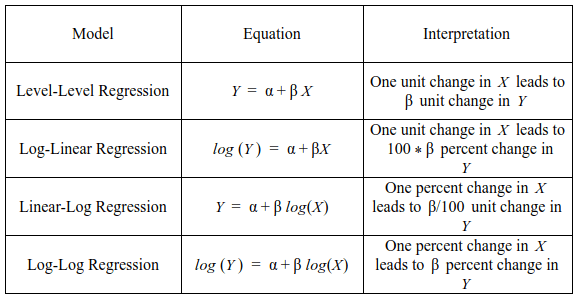
Interpreting Log Transformations

Log transformations of dependent and independent data is an easy way to handle non-linear relationships. The transformation helps to analyze non-linear relationships using linear models. We have discussed the log-linear regression. There are two more variants – a) linear–log regression –the independent variables are log transformed and b) log-log regression – both the dependent and independent variables are transformed. The table below displays the equations and interpretation for each of the models.

Table 2 Sample data for binary logistic regression

Binary Logistic Regression

Binary logistic regression is used when the dependent variable is categorical and takes values - 0 and 1. Unlike simple linear regression, where conditional distribution of dependent variable is normal, in logistic regression the conditional distribution of dependent variable is Bernoulli. In Bernoulli distribution the variable can only take two values – 0 and 1 with certain probabilities.

Lets understand with the help of an example. Let us assume that in football the ability to convert a penalty depends on number of hours of practice by the shooter.  We can represent a successful penalty by 1 and an unsuccessful penalty by 0. The data looks as follows:

Table 2 Sample data for binary logistic regression

The binary logistic regression model will output the probability of successful penalty shoot based on the hours of practice. The logistic regression uses logistic function to model the relationship. Logistic function allows to model the relationship in form of probabilities as it takes values between 0 and 1. It is represented as follows:

[4]

A positive value (negative value) of β1 would indicate that probability of Y=1 increases (decreases) as X increases. Logistic regression is one of the widely used model of class prediction. The multinomial logistic regression extends the binary model to deal with problems involving multiple classes. For example, whether a person will redeem coupon A, coupon B or coupon C. Now we will implement the logistic regression model in R. The sample data consists of two variables – success/ failure in penalty shoot out represent 1/0 and hours of practice. Please click here to download. The R code is follows:

## Prepare scatter plot

#Read data from .csv file
data1 = read.csv("Penalty.csv", header = T)
head(data1)

#Scatter Plot
plot(data1, main = "Scatter Plot")

Figure 4 Scatter plot for categorical data

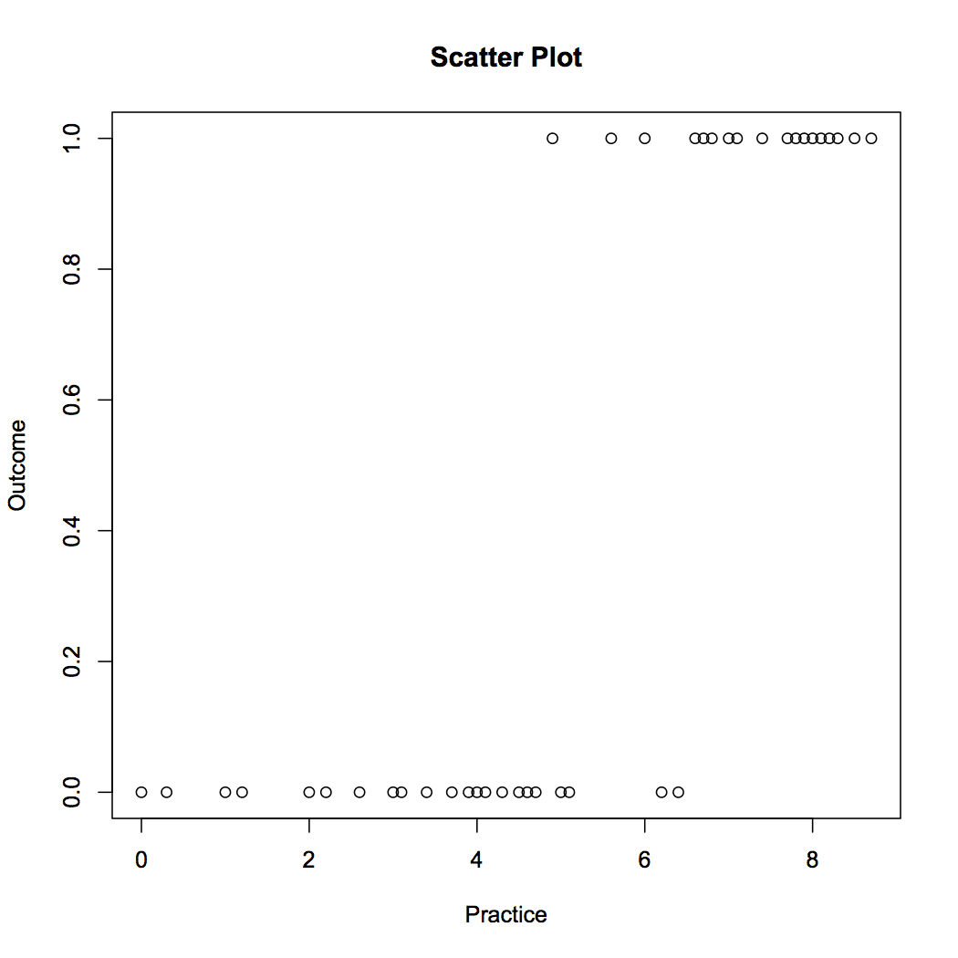
We can observe that the dependent variable can take only two values – 1 and 0. As the number of practice hours increases the efficiency of player increases. Now we will prepare a model using logistic regression to predict the probability of a success or failure based on the practice hours. The R code is as follows:

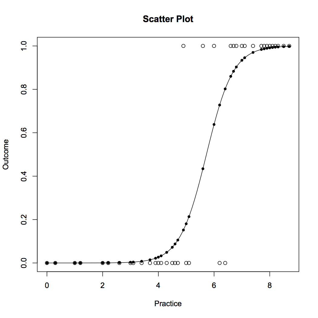
## Fitting Logistic regression model
fit = glm(Outcome ~ Practice, family = binomial(link = "logit"), data = data1)

#Plot probabilities
plot(data1, main ="Scatter Plot")
curve(predict(fit,data.frame(Practice = x), type = "resp"), add = TRUE) 
points(data1$Practice,fitted(fit),pch=20)

Figure 5 displays the probability values obtained from the logistic regression. We can see that the model does a good job. The probability of success increases with increase in practice hours. The model is represented in equation [5]. The probability values can be obtained by plugging in the number of practice hours.

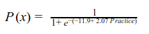[5]

Figure 5 Probability plot using logistic regression

Conclusion

In this article we learned about Generalized Linear Model (GLM). Simple linear regression is the most basic form of GLM. Advance form of GLM helps to deal with non-normal distributions and non-linear relationships in a simple manner. We focus on log-linear regression and binary logistic regression. Log-linear regression is useful when the relation between dependent and independent variable is non-linear. It also provides a quick fix when dependent variable follows log-normal or Poisson distribution.

Further, we discussed the basic concepts of binary logistic regression. Binary logistic regression is beneficial when the dependent variable follows Bernoulli distribution, i.e. can take only values of 0 and 1. We also provide equations and interpretation for various log transformations that are used with regression models.

Along with the theoretical explanation, we share the R codes, so that you can implement the model on R. For better understanding, we display the results along with the codes.

We hope you find the article is useful.

The full code used in this article is provided here.

Bio: Chaitanya Sagar is the Founder and CEO of Perceptive Analytics. Perceptive Analytics has been chosen as one of the top 10 analytics companies to watch out for by Analytics India Magazine. It works on Marketing Analytics for e-commerce, Retail and Pharma companies.

Related:

• Next Generation Data Manipulation with R and dplyr
• A Solution to Missing Data: Imputation Using R
• Python vs R – Who Is Really Ahead in Data Science, Machine Learning?