Process Mining with R: Introduction

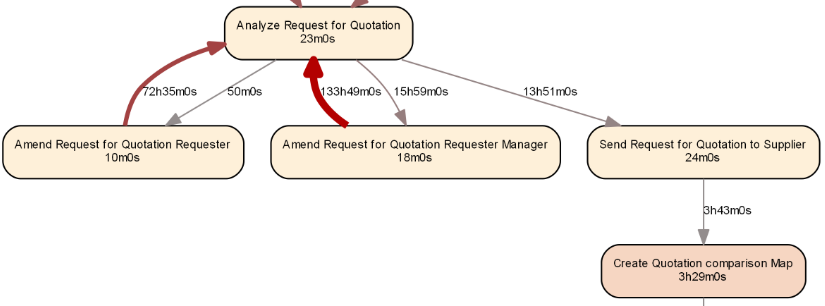
We can then create an igraph object from this information and export it to render it using Graphviz, resulting in the following process map (fragment):

The road is now open for further expansion upon this basic framework and to merge it with predictive and descriptive analytical models. Some ideas for experimentation include:

• Filtering the event log and process map to show high-frequent behavior only
• Playing with different coloring, for instance not based on frequency or performance but also other interesting data attributes
• Expand the framework to include basic conformance checking, e.g. by highlighting deviating flows
• Applying decision mining (or probability measures) on the splits to predict which pathways will be followed

Let’s apply a simple extension as follows: say we’re interested in the “Analyze Request for Quotation” activity and would to bring in some more information with regards to this activity, starting from the resource attribute, the person who has executed this activity.

We hence construct two new data frames for the activities and edges, now using frequency counts as our metric of interest:

col.box.blue <- colorRampPalette(c('#DBD8E0', '#014477'))(20)

col.arc.blue <- colorRampPalette(c('#938D8D', '#292929'))(20)

activities.counts <- activities.basic %>%

select(act) %>%

group_by_all %>%

summarize(metric=n()) %>%

ungroup %>%

mutate(fillcolor=col.box.blue[floor(linMap(metric, 1,20))])

edges.counts <- edges.basic %>%

select(a.act, b.act) %>%

group_by_all %>%

summarize(metric=n()) %>%

ungroup %>%

mutate(color=col.arc.blue[floor(linMap(metric, 1,20))],

penwidth=floor(linMap(metric, 1, 5)),

metric.char=as.character(metric))

Next up, we filter the event log for our activity under interest, calculate the durations, and then calculate frequency and performance metrics for each resource-activity pair that worked on this activity.

acts.res <- eventlog %>%

filter(Activity == "Analyze Request for Quotation") %>%

mutate(Duration=Complete-Start) %>%

select(Duration, Resource, Activity) %>%

group_by(Resource, Activity) %>%

summarize(metric.freq=n(), metric.perf=median(Duration)) %>%

ungroup %>%

mutate(color='#75B779',

penwidth=1,

metric.char=formatSeconds(as.numeric(metric.perf)))

A helpful igraph function to use here is “graph_from_data_frame”. This function expects a data frame of vertices (with all columns except for the first one automatically acting as attributes) and a data frame of edges (with all columns except for the first two acting as attributes). We hence construct a final data frame of vertices (activities) as follows. The fillcolor is set based on whether the node represents an activity (in which case we use the color we set above) or a resource (in which case we use a green color):

a <- bind_rows(activities.counts %>% select(name=act, metric=metric) %>%
mutate(type='Activity'),

acts.res %>% select(name=Resource, metric=metric.freq) %>% 
mutate(type='Resource')) %>%

distinct %>%

rowwise %>%

mutate(fontsize=8,

fontname='Arial',

label=paste(name, metric, sep='\n'),

shape=ifelse(type == 'Activity', 'box', 'ellipse'),

style=ifelse(type == 'Activity', 'rounded,filled', 'solid,filled'),

fillcolor=ifelse(type == 'Activity',
activities.counts[activities.counts$act==name,]$fillcolor, '#75B779'))

And construct a data frame for the edges as well:

e <- bind_rows(edges.counts,

acts.res %>% select(a.act=Resource, b.act=Activity, metric.char, color, penwidth)) %>%

rename(label=metric.char) %>%

mutate(fontsize=8, fontname='Arial')

Finally, we can construct an igraph object as follows:

gh <- graph_from_data_frame(e, vertices=a, directed=T)

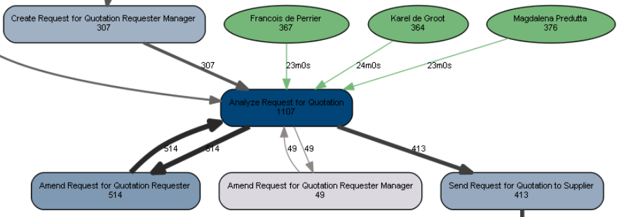
After exporting and plotting this object, we see that all three resources contributed about evenly to the execution of our activity, with their median execution times (shown on the green arcs) being similar as well:

Certainly, we now have a strong framework from which we can start creating richer process maps with more annotations and information embedded.

In this article, we provided a quick whirlwind tour on how to create rich process maps using R.As seen, this can come in helpful in cases where typical process discovery tools might not be available, but also provides hints on how typical process mining tasks can be enhanced by or more easily combined with other more data mining related tasks.We hope you enjoyed reading this article and hope that can’t wait to see what you’ll do with your event logs.

Further reading:

• vanden Broucke S., Vanthienen J., Baesens B. (2013). Volvo IT Belgium VINST. Proceedings of the 3rd Business Process Intelligence Challenge co-located with 9th International Business Process Intelligence workshop (BPI 2013): Vol. 1052. Business Process Intelligence Challenge 2013 (BPIC 2013). Beijing (China), 26 August 2013 (art.nr. 3). Aachen (Germany): RWTH Aachen University.http://ceur-ws.org/Vol-1052/paper3.pdf
• http://www.dataminingapps.com/dma_research/process-analytics/

Bio: Seppe vanden Broucke is an assistant professor at the Faculty of Economics and Business, KU Leuven, Belgium. His research interests include business data mining and analytics, machine learning, process management, and process mining. His work has been published in well-known international journals and presented at top conferences. Seppe’s teaching includes Advanced Analytics, Big Data and Information Management courses. He also frequently teaches for industry and business audiences.

Related:

• Privacy, Security and Ethics in Process Mining
• Process Mining: Where Data Science and Process Science Meet
• Improve your processes – with statistical models