The 8 Neural Network Architectures Machine Learning Researchers Need to Learn

comments

5 — Hopfield Networks

 
Recurrent networks of non-linear units are generally very hard to analyze. They can behave in many different ways: settle to a stable state, oscillate, or follow chaotic trajectories that cannot be predicted far into the future. A Hopfield net is composed of binary threshold units with recurrent connections between them. In 1982, John Hopfield realized that if the connections are symmetric, there is a global energy function. Each binary “configuration” of the whole network has an energy; while the binary threshold decision rule causes the network to settle for a minimum of this energy function. A neat way to make use of this type of computation is to use memories as energy minima for the neural net. Using energy minima to represent memories gives a content-addressable memory. An item can be accessed by just knowing part of its content. It is robust against hardware damage.

Each time we memorize a configuration, we hope to create a new energy minimum. But what if two nearby minima at an intermediate location? This limits the capacity of a Hopfield net. So how do we increase the capacity of a Hopfield net? Physicists love the idea that the math they already know might explain how the brain works. Many papers were published in physics journals about Hopfield nets and their storage capacity. Eventually, Elizabeth Gardnerfigured out that there was a much better storage rule that uses the full capacity of the weights. Instead of trying to store vectors in one shot, she cycled through the training set many times and used the perceptron convergence procedure to train each unit to have the correct state given the states of all the other units in that vector. Statisticians call this technique “pseudo-likelihood.”

There is another computational role for Hopfield nets. Instead of using the net to store memories, we use it to construct interpretations of sensory input. The input is represented by the visible units, the interpretation is represented by the states of the hidden units, and the badness of the interpretation is represented by the energy.

6 — Boltzmann Machine Network

 
A Boltzmann machine is a type of stochastic recurrent neural network. It can be seen as the stochastic, generative counterpart of Hopfield nets. It was one of the first neural networks capable of learning internal representations and is able to represent and solve difficult combinatoric problems.

The goal of learning for Boltzmann machine learning algorithm is to maximize the product of the probabilities that the Boltzmann machine assigns to the binary vectors in the training set. This is equivalent to maximizing the sum of the log probabilities that the Boltzmann machine assigns to the training vectors. It is also equivalent to maximizing the probability that we would obtain exactly the N training cases if we did the following: 1) Let the network settle to its stationary distribution N different time with no external input; and 2) Sample the visible vector once each time.

An efficient mini-batch learning procedure was proposed for Boltzmann Machines by Salakhutdinov and Hinton in 2012.

• For the positive phase, first initialize the hidden probabilities at 0.5, then clamp a data vector on the visible units, then update all the hidden units in parallel until convergence using mean field updates. After the net has converged, record PiPj for every connected pair of units and average this over all data in the mini-batch.
• For the negative phase: first keep a set of “fantasy particles.” Each particle has a value that is a global configuration. Then sequentially update all the units in each fantasy particle a few times. For every connected pair of units, average SiSj over all the fantasy particles.

In a general Boltzmann machine, the stochastic updates of units need to be sequential. There is a special architecture that allows alternating parallel updates which are much more efficient (no connections within a layer, no skip-layer connections). This mini-batch procedure makes the updates of the Boltzmann machine more parallel. This is called a Deep Boltzmann Machine (DBM), a general Boltzmann machine with a lot of missing connections.

In 2014, Salakhutdinov and Hinton came up with another update for their model, calling it Restricted Boltzmann Machines. They restrict the connectivity to make inference and learning easier (only one layer of hidden units and no connections between hidden units). In an RBM it only takes one step to reach thermal equilibrium when the visible units are clamped.

Another efficient mini-batch learning procedure for RBM goes like this:

• For the positive phase, first clamp a data vector on the visible units. Then compute the exact value of <ViHj> for all pairs of a visible and a hidden unit. For every connected pair of units, average <ViHj> over all data in the mini-batch.
• For the negative phase, also keep a set of “fantasy particles.” Then update each fantasy particle a few times using alternating parallel updates. For every connected pair of units, average ViHj over all the fantasy particles.

7 — Deep Belief Network

Back-propagation is considered the standard method in artificial neural networks to calculate the error contribution of each neuron after a batch of data is processed. However, there are some major problems using back-propagation. Firstly, it requires labeled training data; while almost all data is unlabeled. Secondly, the learning time does not scale well, which means it is very slow in networks with multiple hidden layers. Thirdly, it can get stuck in poor local optima, so for deep nets they are far from optimal.

To overcome the limitations of back-propagation, researchers have considered using unsupervised learning approaches. This helps keep the efficiency and simplicity of using a gradient method for adjusting the weights, but also use it for modeling the structure of the sensory input. In particular, they adjust the weights to maximize the probability that a generative model would have generated the sensory input. The question is what kind of generative model should we learn? Can it be an energy-based model like a Boltzmann machine? Or a causal model made of idealized neurons? Or a hybrid of the two?

A belief net is a directed acyclic graph composed of stochastic variables. Using belief net, we get to observe some of the variables and we would like to solve 2 problems: 1) The inference problem: Infer the states of the unobserved variables, and 2) The learning problem: Adjust the interactions between variables to make the network more likely to generate the training data.

Early graphical models used experts to define the graph structure and the conditional probabilities. By then, the graphs were sparsely connected; so researchers initially focused on doing correct inference, not on learning. For neural nets, learning was central and hand-writing the knowledge was not cool, because knowledge came from learning the training data. Neural networks did not aim for interpretability or sparse connectivity to make inference easy. Nevertheless, there are neural network versions of belief nets.

There are two types of generative neural network composed of stochastic binary neurons: 1) Energy-based, in which we connect binary stochastic neurons using symmetric connections to get a Boltzmann Machine; and 2) Causal, in which we connect binary stochastic neurons in a directed acyclic graph to get a Sigmoid Belief Net. The descriptions of these two types go beyond the scope of this article.

8 — Deep Auto-encoders

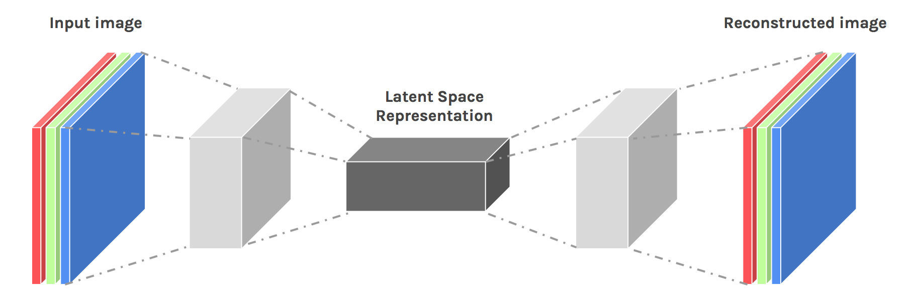
Finally, let’s discuss deep auto-encoders. They always looked like a really nice way to do non-linear dimensionality reduction because of a few reasons: They provide flexible mappings both ways. The learning time is linear (or better) in the number of training cases. And the final encoding model is fairly compact and fast. However, it turned out to be very difficult to optimize deep auto encoders using back propagation. With small initial weights, the back propagated gradient dies. We now have a much better ways to optimize them; either use unsupervised layer-by-layer pre-training or just initialize the weights carefully as in Echo-State Nets.

For pre-training task, there are actually 3 different types of shallow auto-encoders:

1. RBM’s as auto-encoders: When we train an RBM with one-step contrastive divergence, it tries to make the reconstructions look like data. It’s like an auto encoder, but it’s strongly regularized by using binary activities in the hidden layer. When trained with maximum likelihood, RBMs are not like auto encoders. We can replace the stack of RBM’s used for pre-training by a stack of shallow auto encoders; however pre-training is not as effective (for subsequent discrimination) if the shallow auto encoders are regularized by penalizing the squared weights.
2. Denoising auto encoders: These add noise to the input vector by setting many of its components to 0 (like dropout, but for inputs). They are still required to reconstructing these components so they must extract features that capture correlations between inputs. Pre-training is very effective if we use a stack of denoting auto encoders. It’s as good as or better than pre-training with RBMs. It’s also simpler to evaluate the pre-training because we can easily compute the value of the objective function. It lacks the nice variational bound we get with RBMs, but this is only of theoretical interest.
3. Contractive auto encoders: Another way to regularize an auto encoder is to try to make the activities of the hidden units as insensitive as possible to the inputs; but they cannot just ignore the inputs because they must reconstruct them. We achieve this by penalizing the squared gradient of each hidden activity with respect to the inputs. Contractive auto encoders work very well for pre-training. The codes tend to have the property that only a small subset of the hidden units are sensitive to changes in the input.

In brief, there are now many different ways to do layer-by-layer pre-training of features. For datasets that do not have huge numbers of labeled cases, pre-training helps subsequent discriminative learning. For very large, labeled datasets, initializing the weights used in supervised learning by using unsupervised pre-training is not necessary, even for deep nets. Pre-training was the first good way to initialize the weights for deep nets, but now there are other ways. But if we make the nets much larger, we will need pre-training again!

Last Takeaway

Neural networks are one of the most beautiful programming paradigms ever invented. In the conventional approach to programming, we tell the computer what to do, breaking big problems up into many small, precisely defined tasks that the computer can easily perform. By contrast, in a neural network we don’t tell the computer how to solve our problem. Instead, it learns from observational data, figuring out its own solution to the problem at hand.

Today, deep neural networks and deep learning achieve outstanding performance on many important problems in computer vision, speech recognition, and natural language processing. They’re being deployed on a large scale by companies such as Google, Microsoft, and Facebook.

I hope that this post helps you learn the core concepts of neural networks, including modern techniques for deep learning. You can get all the lecture slides, research papers and programming assignments I have done for Dr. Hinton’s Coursera course from my GitHub repo here. Good luck studying!

 
Bio: James Le is currently applying for Master of Science Computer Science programs in the US for the Fall 2018 admission. His intended research will focus on Machine Learning and Data Mining. In the mean time, he is working as a freelance full-stack web developer.

Original. Reposted with permission.

Related:

• The 10 Deep Learning Methods AI Practitioners Need to Apply
• The 10 Algorithms Machine Learning Engineers Need to Know
• The 10 Statistical Techniques Data Scientists Need to Master