Preprocessing for Deep Learning: From covariance matrix to image whitening

comments

2. Preprocessing

 
A. Mean normalization

Mean normalization is just removing the mean from each observation.

where X’ is the normalized dataset, X is the original dataset, and x̅ is the mean of X.

Mean normalization has the effect of centering the data around 0. We will create the function center() to do that:

Let’s give it a try with the matrix B we have created earlier:

Before:

Covariance matrix:
[[ 0.95171641 0.92932561]
 [ 0.92932561 1.12683445]]

After:

Covariance matrix:
[[ 0.95171641 0.92932561]
 [ 0.92932561 1.12683445]]

The first plot shows again the original data B and the second plot shows the centered data (look at the scale).

B. Standardization or normalization

Standardization is used to put all features on the same scale. Each zero-centered dimension is divided by its standard deviation.

where X’ is the standardized dataset, X is the original dataset, x̅ is the mean of X, and σ is the standard deviation of X.

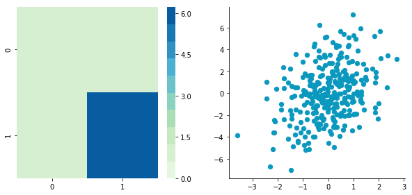
Let’s create another dataset with a different scale to check that it is working.

Covariance matrix:
[[ 0.95171641 0.83976242]
 [ 0.83976242 6.22529922]]

We can see that the scales of x and y are different. Note also that the correlation seems smaller because of the scale differences. Now let’s standardize it:

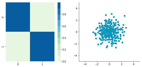
Covariance matrix:
[[ 1.          0.34500274]
 [ 0.34500274  1.        ]]

Looks good. You can see that the scales are the same and that the dataset is zero-centered according to both axes.

Now, have a look at the covariance matrix. You can see that the variance of each coordinate — the top-left cell and the bottom-right cell — is equal to 1.

This new covariance matrix is actually the correlation matrix. The Pearson correlation coefficient between the two variables (c1 and c2) is 0.54220151.

C. Whitening

Whitening, or sphering, data means that we want to transform it to have a covariance matrix that is the identity matrix — 1 in the diagonal and 0 for the other cells. It is called whitening in reference to white noise.

Here are more details on the identity matrix.

Whitening is a bit more complicated than the other preprocessing, but we now have all the tools that we need to do it. It involves the following steps:

• Zero-center the data
• Decorrelate the data
• Rescale the data

Let’s take again C and try to do these steps.

1. Zero-centering

This refers to mean normalization (2. A). Check back for details about the center() function.

Covariance matrix:
[[ 0.95171641  0.83976242]
 [ 0.83976242  6.22529922]]

2. Decorrelate

At this point, we need to decorrelate our data. Intuitively, it means that we want to rotate the data until there is no correlation anymore. Look at the following image to see what I mean:

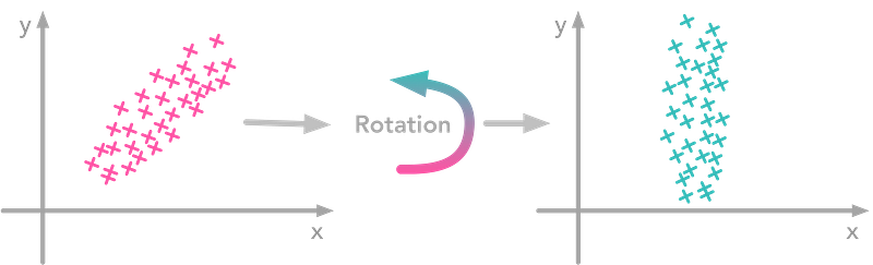
The left plot shows correlated data. For instance, if you take a data point with a big x value, chances are that the associated y will also be quite big.

Now take all data points and do a rotation (maybe around 45 degrees counterclockwise. The new data, plotted on the right, is not correlated anymore. You can see that big and small y values are related to the same kind of x values.

The question is: how could we find the right rotation in order to get the uncorrelated data?

Actually, it is exactly what the eigenvectors of the covariance matrix do. They indicate the direction where the spread of the data is at its maximum:

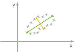
The eigenvectors of the covariance matrix give you the direction that maximizes the variance. The direction of the green line is where the variance is maximum. Just look at the smallest and largest point projected on this line — the spread is big. Compare that with the projection on the orange line — the spread is very small.

For more details about eigendecomposition, see this post.

So we can decorrelate the data by projecting it using the eigenvectors. This will have the effect to apply the rotation needed and remove correlations between the dimensions. Here are the steps:

• Calculate the covariance matrix
• Calculate the eigenvectors of the covariance matrix
• Apply the matrix of eigenvectors to the data — this will apply the rotation

  Let’s pack that into a function:

Let’s try to decorrelate our zero-centered matrix C to see it in action:

Covariance matrix:
[[ 0.95171641 0.83976242]
 [ 0.83976242 6.22529922]]

Covariance matrix:
[[ 5.96126981e-01 -1.48029737e-16]
 [ -1.48029737e-16 3.15205774e+00]]

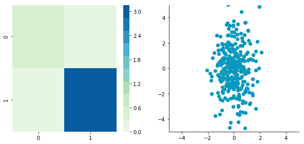
Nice! This is working.

We can see that the correlation is not here anymore. The covariance matrix, now a diagonal matrix, confirms that the covariance between the two dimensions is equal to 0.

3. Rescale the data

The next step is to scale the uncorrelated matrix in order to obtain a covariance matrix corresponding to the identity matrix.To do that, we scale our decorrelated data by dividing each dimension by the square-root of its corresponding eigenvalue.

Note: we add a small value (here 10^-5) to avoid division by 0.

Covariance matrix:
[[ 9.99983225e-01 -1.06581410e-16]
 [ -1.06581410e-16 9.99996827e-01]]

Hooray! We can see that with the covariance matrix that this is all good. We have something that looks like an identity matrix — 1 on the diagonal and 0 elsewhere.