Logistic Regression: A Concise Technical Overview

We have all heard of Linear Regression. It’s what we all learn in our first semester of statistics. It is our default technique when we have a continuous outcome variable. A refresher on Linear Regression can be found here. But other times we have Categorical Outcomes. Logistic Regression solves the limitation of Linear Regression in which the outcome variable (y) must be continuous.

Logistic Regression is a Regression technique that is used when we have a categorical outcome (2 or more categories). This technique can be used to analyze and predict variables that are ‘Discrete’, ‘Nominal’ and ‘Ordered’. Logistic Regression is one of the most easily interpretable classification techniques in a Data Scientist’s portfolio.

Unlike Linear Regression, Logistic Regression does not make any assumptions of Normality, Linearity and Homogenity of Variance. This is one of the reasons that Logistic Regression could be more powerful as these assumptions are rarely or if ever satisfied in the real world.

Source: Scikit-learn documentation

An easy way to think of the difference between Linear and Logistic Regression is in Linear Regression, a person can predict a student’s test score (continuous target). In Logistic Regression, a person can assign ‘Pass’, ‘Fail’ categories to student’s scores and predict whether a student passed or failed.

 

Types of Logistic Regression

 

• Binary
• Multinomial
• Ordinal

 
Binary Logistic Regression

The most basic type of Logistic Regression is the Binary Logistic Regression inwhich there are only 2 categorical outcomes.

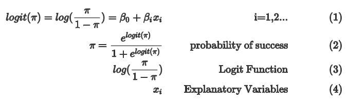
• The Logit function (3) is used to obtain a positive probability value for the target outcome. It is expressed in terms of the log odds of success compared to failure.
  • π (2) is the probability of success.
  • 1-π refers to the probability of failure.
• The Explanatory variables (4) can be categorical or numeric and expressed in terms of the change in log odds of the target outcome.

It is interpreted in the following manner:

Continuous Explanatory Variables

• An increase in the odds of x_i by 1 will increase/decrease the odds of success by e^β_i holding all other variables constant.

Categorical Explanatory Variable

• At level x_i the odds will increase/decrease by e^β₁ more than the reference level holding all other variables constant.

 
Multinomial Logistic Regression

While binary logistic regression will allow us to analyze binary categories as a target variable, other times you will see that the target variables will have more than 2 categories.

eg:

• Apples, Oranges, Grapes, Bananas
• Heart attack, Diabetes, Cancer

Multinomial Regression is used to calculate the odds of a target category relative to a SPECIFIED BASELINE.

In the following equations:

• p refers to a variable / feature / column
• j refers to the category level of the target variable.

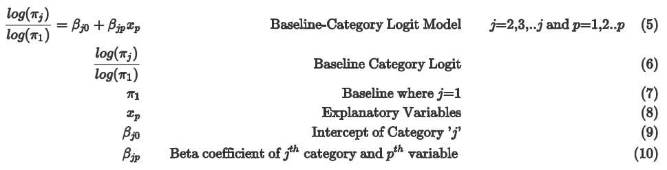
• The baseline model logit (5 & 6) shows us that the predicted probability value is the log odds of log probability _j (log(π_j)) relative to the selected baseline log probability (log(π₁)).
• Each category level 'j ' will have its own intercept (8) and Explanatory variables (7).
• Each Explanatory variable (7) will have its own beta coefficient (9).

It is interpreted in the following manner:

Intercept for j^th level (β_j⁰)

• When all Explanatory variables are zero, the odds of the j^th level is e^β_j0 holding all other variables constant.

Continuous explanatory variables

• When x_p increases by 1 unit, the odds of π_j relative to π₁ changes by e^β_jp holding all other variables constant.

Categorical explanatory variables

• At level x_p, the odds of π_j relative to π_i will increase/decrease by e^β_jp more than the reference level holding all other variables constant.

 
Ordinal Logistic Regression

Ordinal Regression can be seen as an extension from Multinomial Regression. Ordinal Regression can also handle regression problems with more than 2 target levels and in addition to target levels that have a NATURAL ORDER.

eg:

• Ranking scales (1,2,3,4,5)
• High, Low, Medium

• Each target level as its own Intercept ‘β_j0’.
• Explanatory variables are shared among each intercept.
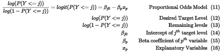
• As we can see in (12) and (13), Ordinal Regression can be used to calculate cumulative probabilities instead of just the probability of a single target.

It is interpreted in the following manner:

Intercept for the j^th level (β_j0)

• When all explanatory variables are zero, the odds of the j^th level is e^β_j0 holding all other variables constant.

Continuous explanatory variables

• When x_p increases by 1 unit, the odds of (12) relative to (13) changes by e^β_p holding all other variables constant.

Categorical explanatory variables

• At level x_p, the odds of (12) relative to (13) will increase/decrease by e^β_p more than the reference level holding all other variables constant.

For Ordinal Regression, P(Y <= j) will refer to the target level desired by the user and 1 - P(Y <= j) refers to the remaining category levels.

 

Conclusion

 
Logistic Regressions are some of the most simple but powerful techniques in Machine Learning. The different forms of Logistic Regression can be used to model many real world scenarios with a relatively easily interpretable outcome. This is not a black-box process which adds to its attractiveness to be used. Many believe Logistic Regression to be used only with binary outcomes but as we have seen it is not the case.

A great reason to gain a deep understanding of Logistic Regression is that it helps to understand Neural Networks. Machine Learning is at its core the method of computers making decisions and many decisions are categorical/discrete in nature. Learning Logistic Regression can be a segue to understanding Neural Networks.

Most of the information in this article can be found with corresponding R codes here for each type of Logistic Regression.

 
Related:

• 5 Reasons Logistic Regression should be the first thing you learn when becoming a Data Scientist
• A Primer on Logistic Regression – Part I
• Regularization in Logistic Regression: Better Fit and Better Generalization?