Naive Bayes: A Baseline Model for Machine Learning Classification Performance

Multinomial Naive Bayes

First, the categorical variables will need to be encoded.

o = {'sunny': 1, 'overcast': 2, 'rainy': 3}
data.outlook = [o[item] for item in data.outlook.astype(str)]

t = {'hot': 1, 'mild': 2, 'cool': 3}
data.temp = [t[item] for item in data.temp.astype(str)]

h = {'high': 1, 'normal': 2}
data.humidity = [h[item] for item in data.humidity.astype(str)]

w = {'True': 1, 'False': 2}
data.windy = [w[item] for item in data.windy.astype(str)]

Then we can create our training and test sets

x = tennis.iloc[:,0:-1] # X is the features in our dataset
y = tennis.iloc[:,-1]   # y is the Labels in our dataset

X_train, X_test, y_train, y_test = train_test_split(x, y, test_size=0.33, random_state=42)

Next, we can go on to fit our model and make predictions

modelM = MultinomialNB().fit(X_train, y_train)
predM = model.predict(X_test)
predM

array(['yes', 'yes', 'yes', 'yes', 'yes'], dtype='<U3')

It seems that the predictions have all returned 'yes'. This will have implications when evaluating the model as you will see.

Lets make a confusion matrix with pandas as I personally do not like the confusion matrix in Scikitlearn.

pd.crosstab(y_test, predy, rownames=['Actual'], colnames=['Predicted'], margins=True)

    Predicted 	yes All
Actual
no 	         2  2
yes 	         3  3
All 	         5  5

accuracy_score = accuracy_score(y_test, predy)
print('The accuracy of the Multinomial model is ', accuracy_score)

The accuracy of the Multinomial model is 0.6

The Multinomaial model gives us an accuracy of 60%
The RECALL (TRUE POSITIVE RATE) for the model is 100% due to there being no false negatives as there were no '0' classes predicted. Recall is calculated by [True positive/(True Positive+False Negative)]. Unfortunately, this is not acceptable because it unfathomable to have a 100% recall in a real world situation. This is merely the mathematics at play that require human interpretation to assess its suitability.

Gaussian Naive Bayes

As the Gaussian Naive Bayes prefers continuous data, we are going to use the Pima Indians Diabetes datset

diabetes = pd.read_csv('diabetes.csv')

diabetes.dtypes

  Pregnancies                   int64
  Glucose                       int64
  BloodPressure                 int64
  SkinThickness                 int64
  Insulin                       int64
  BMI                         float64
  DiabetesPedigreeFunction    float64
  Age                           int64
  Outcome                       int64
  dtype: object

As we can see all the features are continuous.

Now lets test to see whether the features follow a Gaussian Distribution (Normal Distribution) as it is a required assumption of the Gaussian Naive Bayes model (although it can still be used if the data is not normally distributed)

The loop will tell us whether the data is normally distributed using the famous Shapiro-Wilkes test.

  for i in range(0,9):
      stat,p = shapiro(diabetes[diabetes.columns[i]])
      print(diabetes.columns[i], 'Test-Statistic=%.3f, p-value=%.3f' % (stat, p));
      alpha = 0.05
      if p > alpha:
          print(diabetes.columns[i], 'looks Gaussian (fail to reject H0)')
          print('---------------------------------------')
      else:
          print(diabetes.columns[i],'does not look Gaussian (reject H0)')
          print('---------------------------------------')

  Pregnancies Test-Statistic=0.904, p-value=0.000
  Pregnancies does not look Gaussian (reject H0)
  ---------------------------------------
  Glucose Test-Statistic=0.970, p-value=0.000
  Glucose does not look Gaussian (reject H0)
  ---------------------------------------
  BloodPressure Test-Statistic=0.819, p-value=0.000
  BloodPressure does not look Gaussian (reject H0)
  ---------------------------------------
  SkinThickness Test-Statistic=0.905, p-value=0.000
  SkinThickness does not look Gaussian (reject H0)
  ---------------------------------------
  Insulin Test-Statistic=0.722, p-value=0.000
  Insulin does not look Gaussian (reject H0)
  ---------------------------------------
  BMI Test-Statistic=0.950, p-value=0.000
  BMI does not look Gaussian (reject H0)
  ---------------------------------------
  DiabetesPedigreeFunction Test-Statistic=0.837, p-value=0.000
  DiabetesPedigreeFunction does not look Gaussian (reject H0)
  ---------------------------------------
  Age Test-Statistic=0.875, p-value=0.000
  Age does not look Gaussian (reject H0)
  ---------------------------------------
  Outcome Test-Statistic=0.603, p-value=0.000
  Outcome does not look Gaussian (reject H0)
  ---------------------------------------

None of the features appear to be normally distributed.

Lets take it one step further and visualize their distributions

diabetes.hist(figsize=(20, 10));

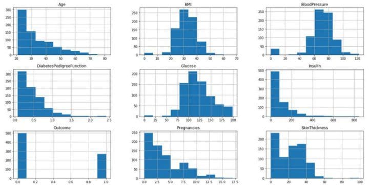
Upon visual inspection BMI and Blood Pressure seem to follow a normal distribution but the outliers on either side and the hypothesis test will have us think otherwise. Although the assumption
does not hold, we can still move forward to fit the model.

  xG = diabetes.iloc[:,0:-1] # X is the features in our dataset
  yG = diabetes.iloc[:,-1]   # y is the Labels in our dataset

  X_trainG, X_testG, y_trainG, y_testG = train_test_split(xG, yG, test_size=0.33, random_state=42)

modelG = GaussianNB().fit(X_trainG, y_trainG)
predG = modelG.predict(X_testG)

pd.crosstab(y_testG, predG, rownames=['Actual'], colnames=['Predicted'], margins=True)

    Predicted 	0 	1 	All
Actual
0 	        136 	32 	168
1             	33 	53 	86
All 	        169 	85 	254

This time we can compute a Recall (True Positive Rate) as now both classes have been predicted.

recall = recall_score(y_testG, predG, average='binary')
print('The Recall of the Gaussian model is', recall)

The Recall of the Gaussian model is 0.6162790697674418

I use average='binary' because our target variable is a binary target (0 and 1).
The model gives us a True Positive Rate (Recall) of 62%.

I had trouble obtaining the Accuracy for the model so we can just compute it manually:

tn, fn, fp, tp = confusion_matrix(y_testG, predG).ravel()
accuracy = (tp + tn) /(tp+fp+tn+fn)
print('The accuracy of the Gaussian model is', accuracy)

The accuracy of the Gaussian model is 0.7440944881889764

The Gaussian model gives us 74% accuracy

Advantages of Naive Bayes

1. Can handle missing values
   • Missing values are ignored while preparing the model and ignored when a probability is calculated for a class value.
2. Can handle small sample sizes.
   • Naive Bayes does not require a large amount of training data. It merely needs enough data to understand the probabilistic relationship between each attribute in isolation with the target variable. If only little training data is available, Naive Bayes would usually perform better than other models.
3. Performs well despite violation of independence assumption
   • Even though independence rarely holds for real world data, the model will still perform as usual.
4. Easily interpretable and has fast prediction time in comparison.
   • Naive Bayes is not a black-box algorithm and the end result can be easily interpreted to an audience.
5. Can handle both numeric and categorical data.
   • Naive Bayes is a classifier and will therefore perform better with categorical data. Although numeric data will also suffice, it assumes all numeric data are normally distributed which is unlikely in real world data.

Disadvantages of Naive Bayes

1. Naive Assumption
   • Naive Bayes assumes that all features are independent of each other. In real life it is almost impossible to obtain a set of predictors that are completely independent of each other.
2. Cannot incorporate interactions between the features.
3. The model's performance will be highly sensitive to skewed data.
   • When the training set is not representative of the class distributions of the overall population, the prior estimates will be incorrect.
4. Zero Frequency problem
   • Categorical variables that have a category in the test data but was not in the training data will be assigned a probability of zero (0) and will be unable to make a prediction.
   • As a solution, a smoothing technique must be applied to the category. One of the simplest and most famous techniques is the Laplace Smoothing Technique. Python's Sklearn implements laplace smoothing by default.
5. Correlated features in the dataset must be removed or else are voted twice in the model and will over-inflate the importance of that feature.

Why use Naive Bayes as a baseline Classifier for performance?

My thoughts as to why Naive Bayes should be the first model to create and compare is that:

• It heavily relies on the prior target class probability for predictions. Inaccurate or unrealistic priors can lead to misleading results. Because Naive Bayes is a probability based machine learning technique, the probability of the target will greatly affect the final prediction.
• Since you do not have to remove missing values, you will not have to risk losing any of your original data.
• The independence assumption is practically never satisfied and therefore the results are not very trustworthy since its most basic assumption is flawed.
• Interactions between features are not accounted for in the model. However features in the real world almost always have interactions.
• There is no error or variance to minimize but only to seek the higher probability of a class given the predictors.

All of the above can be used as valid points that other classifiers should be built to outperform the Naive Bayes model. While Naive Bayes is great for spam filtering and Recommendation Systems, it is probably not ideal in most other applications.

Conclusion

Overall Naive Bayes is fast, powerful and interpretable. However, the overreliance on the prior probability of the target variable can create very misleading and inaccurate results. Classifiers such as Decision Trees, Logistic Regression, Random Forests and Ensemble methods should be able to outperform Naive bayes to be an actually useful. This is is no way removes Naive Bayes as a powerful classifier. The independence assumption, inability to handle interactions, and gaussian distribution assumption make it a very difficult algorithm to trust with prediction on its own as these models will have to be continuously upated.

Related:

• Naive Bayes from Scratch using Python only – No Fancy Frameworks
• Machine Learning Finds “Fake News” with 88% Accuracy
• Unfolding Naive Bayes From Scratch