Simple clustering methods such as k-means may not be as sexy as contemporary neural networks or other recent advanced non-linear classifiers, but they certainly have their utility, and knowing how to correctly approach an unsupervised learning problem is a great skill to have at your disposal.

This is intended to be the first in a series of articles looking at the different aspects of a k-means clustering pipeline. In this first article we will discuss centroid initialization: what it is, what it accomplishes, and some of the different approaches that exist. We will assume familiarity with machine learning, Python programming, and the general idea of clustering.

k-means Clustering

 
k-means is a simple, yet often effective, approach to clustering. Traditionally, k data points from a given dataset are randomly chosen as cluster centers, or centroids, and all training instances are plotted and added to the closest cluster. After all instances have been added to clusters, the centroids, representing the mean of the instances of each cluster are re-calculated, with these re-calculated centroids becoming the new centers of their respective clusters.

At this point, all cluster membership is reset, and all instances of the training set are re-plotted and re-added to their closest, possibly re-centered, cluster. This iterative process continues until there is no change to the centroids or their membership, and the clusters are considered settled.

Convergence is achieved once the re-calculated centroids match the previous iteration’s centroids, or are within some preset margin. The measure of distance is generally Euclidean in k-means, which, given 2 points in the form of (x, y), can be represented as:

Of technical note, especially in the era of parallel computing, iterative clustering in k-means is serial in nature; however, the distance calculations within an iteration need not be. Therefore, for sets of a significant size, distance calculations are a worthy target for parallelization in the k-means clustering algorithm.

Centroid Initialization Methods

 
As k-means clustering aims to converge on an optimal set of cluster centers (centroids) and cluster membership based on distance from these centroids via successive iterations, it is intuitive that the more optimal the positioning of these initial centroids, the fewer iterations of the k-means clustering algorithms will be required for convergence. This suggests that some strategic consideration to the initialization of these initial centroids could prove useful.

What methods of centroid initialization exist? While there are a number of initialization strategies, let's focus on the following:

• random data points: In this approach, described in the "traditional" case above, k random data points are selected from the dataset and used as the initial centroids, an approach which is obviously highly volatile and provides for a scenario where the selected centroids are not well positioned throughout the entire data space.
• k-means++: As spreading out the initial centroids is thought to be a worthy goal, k-means++ pursues this by assigning the first centroid to the location of a randomly selected data point, and then choosing the subsequent centroids from the remaining data points based on a probability proportional to the squared distance away from a given point's nearest existing centroid. The effect is an attempt to push the centroids as far from one another as possible, covering as much of the occupied data space as they can from initialization. k-means++ original paper, from 2006, can be read here.
• naive sharding: This lesser known (unknown?) centroid initialization method was the subject of some of my own graduate research. It is primarily dependent on the calculation of a composite summation value reflecting all of the attribute values of an instance. Once this composite value is computed, it is used to sort the instances of the dataset. The dataset is then horizontally split into k pieces, or shards. Finally, the original attributes of each shard are independently summed, their mean is computed, and the resultant collection of rows of shard attribute mean values becomes the set of centroids to be used for initialization. The expectation is that, as a deterministic method, it should perform much quicker than stochastic methods, and approximate the spread of initial centroids across the data space via the composite summation value. You can read more about it here if interested.

Variants of any of these are possible: you could randomly select from anywhere in the data space, as opposed to just the space which contains existing data points; you could attempt to find the most centrally located data point first, as opposed to a random selection, and proceed with k-means++ from there; you could swap the post-summation mean operation for an alternate in naive sharding.

Also, a form of hierarchical clustering (often Ward's method) can be used as a method to find the initial cluster centers, which can then be passed off to k-means for the actual data clustering task. This can be effective, but since it would mean also discussing hierarchical clustering we will leave this until a later article.

Centroid Initialization and Scikit-learn

 
As we will use Scikit-learn to perform our clustering, let's have a look at its KMeans module, where we can see the following written about available centroid initialization methods:

init{‘k-means++’, ‘random’, ndarray, callable}, default=’k-means++’

Method for initialization:

'k-means++': selects initial cluster centers for k-mean clustering in a smart way to speed up convergence. See section Notes in k_init for more details.

'random': choose n_clusters observations (rows) at random from data for the initial centroids.

If an ndarray is passed, it should be of shape (n_clusters, n_features) and gives the initial centers.

If a callable is passed, it should take arguments X, n_clusters and a random state and return an initialization.

 
With this in mind, and since we want to be able to compare and inspect initialized centroids — which we are not able to do with Scikit-learn's implementations — we will use our own implementations of the 3 methods discussed above, namely random centroid initialization, k-means++, and naive sharding. We can then use our implementations independent of Scikit-learn to create our centroids, and pass them in as an ndarray at the time of clustering. We could also use the callable option, as opposed to the ndarray option, and integrate the centroid initialization into the Scikit-learn k-means execution, but that puts us right back to square one with not being able to examine and compare these centroids prior to clustering.

With that said, the centroid_initialization.py file contains our centroid initialization implementations.

With this file placed in the same directory as where I have started Jupyter notebook, I can proceed as follows, starting with imports.

import numpy as np
import pandas as pd
import matplotlib.pyplot as plt

from sklearn.cluster import KMeans
import centroid_initialization as cent_init

%matplotlib inline

Creating Some Data

 
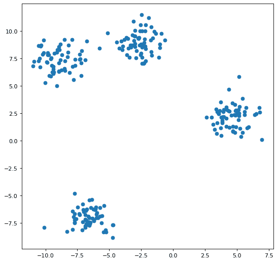
Clearly we will need some data. We will create a small synthetic set in order to have control over clearly delineating our clusters (see Figure 1).

from sklearn.datasets import make_blobs

n_samples = 250
n_features = 2
n_clusters = 4
random_state = 42
max_iter = 100

X, y = make_blobs(n_samples=n_samples, 
                  n_features=n_features, 
                  centers=n_clusters, 
                  random_state=random_state)

fig=plt.figure(figsize=(8,8), dpi=80, facecolor='w', edgecolor='k')
plt.scatter(X[:, 0], X[:, 1]);

Figure 1: Our synthetic dataset

Initializing the Centroids

 
Let's initialize some centroids, using the implementation from above.

Random Initialization

random_centroids = cent_init.random(X, n_clusters)
print(random_centroids)

[[-7.09730839 -5.78133274]
 [ 4.56277713  2.31432166]
 [ 4.9976662   2.53395421]
 [ 4.16493353  1.31984045]]

k-means++ Initialization

plus_centroids = cent_init.plus_plus(X, n_clusters)
print(plus_centroids)

[[-1.59379551  9.34303724]
 [-6.63466062 -7.38705277]
 [-7.31520368  7.86243296]
 [ 5.1549141   2.48695563]]

Naive Sharding Initialization

naive_centroids = cent_init.naive_sharding(X, n_clusters)
print(naive_centroids)

[[-9.09917527 -7.00640594]
 [-6.48108313  2.12605542]
 [-2.66275228  7.07500918]
 [ 4.66778007  9.47156226]]

As you can see, the sets of initialized centroids differ from each other.

Visualizing Centroid Initialization

 
Let's see how our centroids compare to each other, and to the data points, visually. We will call the plotting function below a number of subsequent times for comparison. Figure 2 plots the the 3 sets of centroids created above against the data points.

def centroid_plots(X, rand, plus, naive):
    fig=plt.figure(figsize=(8,8), dpi=80, facecolor='w', edgecolor='k')
    
    plt.scatter(X[:, 0], X[:, 1],
                s=50,
                marker='o',
                label='cluster 1')

    plt.scatter(rand[:, 0], 
                rand[:, 1],
                s=200, c='yellow',
                marker='p')

    plt.scatter(plus[:, 0],
                plus[:, 1],
                s=200, c='red',
                marker='P')

    plt.scatter(naive[:, 0], 
                naive[:, 1],
                s=100, c='green',
                marker='D');

centroid_plots(X, random_centroids, plus_centroids, naive_centroids)

Figure 2. Centroids plotted against data points: random (yellow), k-means++ (red), naive sharding (green)

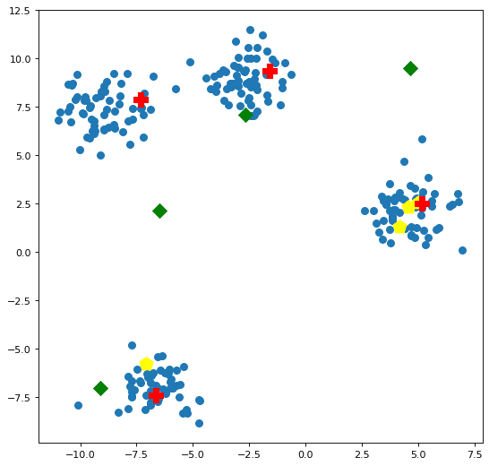
Of note, the luck of the draw has placed 3 of the randomly initialized centroids in the right-most cluster; the k-means++ initialized centroids are located one in each of the clusters; and the naive sharding centroids ended up spread across the data space in a somewhat arcing fashion upward and to the right across the data space, skewed toward where the data is heavily clustered.

Keep in mind that we created a 2 dimensional data space, so the visualization of these centroids is accurate; we aren't stripping away a number of dimensions and artificially plotting the data in a stripped-down space which may be problematic. This means the comparison of the centroids in this case is as accurate as is possible.

You may be asking, what of this initialization is affected by random seeding? Both random initialization and and k-means++ are stochastic methods, and so they can be affected by random seeds. If we pass some different seeds to additional runs of the initialization algorithms, the results are visualized in Figure 3.

Figure 3. Experimenting with random seeds for centroid initialization, clockwise from top left: 123, 249, 127, 13

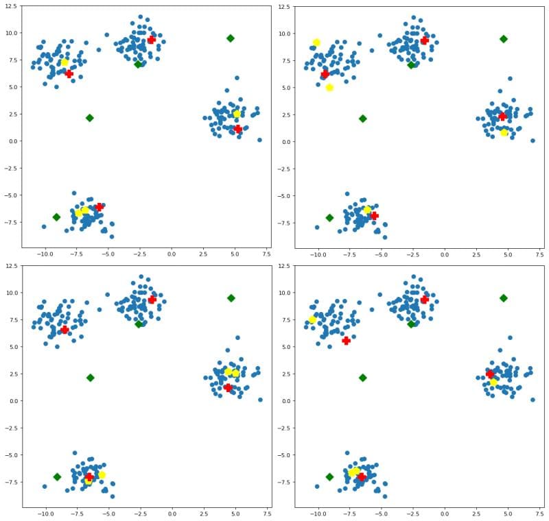
Some observations:

• random initialization is (fittingly) all over the place
• k-means++ is relatively consistent within clusters, with the specific data points selected as initial centroids varying slightly
• naive sharding is deterministic, and so is not affected by seeding

 
This leads us to some questions, which relate directly to the next steps in clustering:

• What effect does centroid placement have on the resulting clustering task?
• What effect does the centroid placement have on the speed of the resulting clustering task?
• What effect does the centroid placement have on the accuracy of the resulting clustering task?
• When would we use certain of these initialization methods over others?
• If random seems as though it might be such a poor initialization method from an optimal placement standpoint, why is it used?
• Is there any advantage to a deterministic initialization method, like naive sharding?

 
We will start searching out the answers to these next time.

 
 
Matthew Mayo (@mattmayo13) is a Data Scientist and the Editor-in-Chief of KDnuggets, the seminal online Data Science and Machine Learning resource. His interests lie in natural language processing, algorithm design and optimization, unsupervised learning, neural networks, and automated approaches to machine learning. Matthew holds a Master's degree in computer science and a graduate diploma in data mining. He can be reached at editor1 at kdnuggets[dot]com.