Essential Math for Data Science: Information Theory

The field of information theory studies the quantification of information in signals. In the context of machine learning, some of these concepts are used to characterize or compare probability distributions. The ability to quantify information is also used in the decision tree algorithm, to select the variables associated with the maximum information gain. The concepts of entropy and cross-entropy are also important in machine learning because they lead to a widely used loss function in classification tasks: the cross-entropy loss or log loss.

Shannon Information

 
Intuition
The first step to understanding information theory is to consider the concept of quantity of information associated with a random variable. In information theory, this quantity of information is denoted as II and is called the Shannon information, information content, self-information, or surprisal. The main idea is that likely events convey less information than unlikely events (which are thus more surprising). For instance, if a friend from Los Angeles, California tells you: “It is sunny today”, this is less informative than if she tells you: “It is raining today”. For this reason, is can be helpful to think of the Shannon information as the amount of surprise associated with an outcome. You’ll also see in this section why it is also a quantity of information, and why likely events are associated with less information.

Units of Information

Common units to quantity information are the nat and the bit. These quantities are based on logarithm functions. The word nat, short for natural unit of information is based on the natural logarithm, while the bit, short for “binary digit”, is based on base-two logarithms. The bit is thus a rescaled version of the nat. The following sections will mainly use the bit and base-two logarithms in formulas, but replacing it with the natural logarithm would just change the unit from bits to nats.

Bits represent variables that can take two different states (0 or 1). For instance, 1 bit is needed to encode the outcome of a coin flip. If you flip two coins, you’ll need at least two bits to encode the result. For instance, 00 for HH, 01 for HT, 10 for TH and 11 for TT. You could use other codes, such as 0 for HH, 100 for HT, 101 for TH and 111 for TT. However, this code uses a larger number of bits in average (considering that the probability distribution of the four events is uniform, as you’ll see)

Let’s take an example to see what a bit describes. Erica sends you a message containing the result of three coin flips, encoding ‘heads’ as 0 and ‘tails’ as 1. There are 8 possible sequences, such as 001, 101, etc. When you receive a message of one bit, it divides your uncertainty by a factor of 2. For instance, if the first bit tells you that the first roll was ‘heads’, the remaining possible sequences are 000, 001, 010, and 011. There are only 4 possible sequences instead of 8. Similarly, receiving a message of two bits will divide your uncertainty by a factor of 2222; a message of three bits, by a factor of 2323, and so on.

Note that we talk about “useful information”, but it is possible that the message is redundant and convey less information with the same number of bits.

Example

Let’s say that we want to transmit the result of a sequence of eight tosses. You’ll allocate one bit per toss. You thus need eight bits to encode the sequence. The sequence might be for instance “00110110”, corresponding to HHTTHTTH(four “heads” and four “tails”).

However, let’s say that the coin is biased: the chance to get “tails” is only 1 over 8. You can find a better way to encode the sequence. One option is to encode the index of the outcomes “tails”: it will take more than one bit, but ‘tails’ occurs only for a small proportion of the trials. With this strategy, you allocate more bits to rare outcomes.

This example illustrates that more predictable information can be compressed: a biased coin sequence can be encoded with a smaller amount of information than a fair coin. This means that Shannon information depends on the probability of the event.

Mathematical Description

Shannon information encodes this idea and converts the probability that an event will occur into the associated quantity of information. Its characteristics are that, as you saw, likely events are less informative than unlikely events and also that information from different events is additive (if the events are independent).

Mathematically, the function I(x) is the information of the event X=x that takes the outcome as input and returns the quantity of information. It is a monotonically decreasing function of the probability (that is, a function that never increases when the probability increases). Shannon information is described as:

The result is a lower bound on the number of bits, that is, the minimum amount of bits needed to encode a sequence with an optimal encoding.

The logarithm of a product is equal to the sum of the elements: . This property is useful to encode the additive property of the Shannon information. The probability of occurrence of two events is their individual probabilities multiplied together (because they are independent, as you saw in Essential Math for Data Science):

This means that the information corresponding to the probability of occurrence of two events P(x,y) equals the information corresponding to P(x) added to the information corresponding to P(y). The information of independent events add together.

Let’s plot this function for a range of probability between 0 and 1 to see the shape of the curve:

plt.plot(np.arange(0.01, 1, 0.01), -np.log2(np.arange(0.01, 1, 0.01)))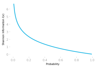

Figure 1: The quantity of information is given by the negative logarithm of the probability.

As you can see in Figure 1, the negative logarithm function encodes the idea that a very unlikely event (probability around 0) is associated with a large quantity of information and a likely event (probability around 1) is associated with a quantity of information around 0.

Since you used a base-two logarithm np.log2(), the information I(x) is measured in bits.

Entropy

 
You saw that Shannon information gives the amount of information associated with a single probability. You can also calculate the amount of information of a discrete distribution with the Shannon entropy, also called information entropy, or simply entropy.

Example

Consider for instance a biased coin, where you have a probability of 0.8 of getting ‘heads’.

1. Here is your distribution: you have a probability of 0.8 of getting ‘heads’ and a probability of 1 − 0.8 = 0.2 of getting ‘tails’.
2. These probabilities are respectively associated with a Shannon information of:

and

1. Landing ‘heads’ is associated with an information around 0.32 and landing ‘tails’ to 2.32. However, you don’t have the same number of ‘heads’ and ‘tails’ in average, so you must weight the Shannon information of each probability with the probability itself. For instance, if you want to transmit a message with the results of, say, 100 trials, you’ll need around 20 times the amount of information corresponding to ‘tails’ and 80 times the amount of information corresponding to ‘heads’. You get:

and

1. The sum of these expressions gives you:

The average number of bits required to describe a series of events from this distribution is 0.72 bits.

To summarize, you can consider the entropy as a summary of the information associated with the probabilities of the discrete distribution:

1. You calculate the Shannon information of each probability of your distribution.
2. You weight the Shannon information with the corresponding probability.
3. You sum the weighted results.

Mathematical Formulation

The entropy is the expectation of the information with respect to the probability distribution. Remember from Essential Math for Data Science that the expectation is the mean value you’ll get if you draw a large number of samples from the distribution:

with the random variable X having n possible outcomes, x_i being the ith possible outcome corresponding to a probability of P(x_i). The expected value of the information of a distribution corresponds to the average of the information you’ll get.

Following the formula of the expectation and the Shannon information, the entropy of the random variable X is defined as:

The entropy gives you the average quantity of information that you need to encode the states of the random variable X.

Note that the input of the function H(X) is the random variable X while I(x) denotes the Shannon information of the event X=x. You can also refer to the entropy of the random variable X which is distributed with respect to P(x) as H(P).

Illustration

Let’s take an example: as illustrated in Figure 2 in the bottom panel, you have a discrete distribution with four possible outcomes, associated with probabilities 0.4, 0.4, 0.1, and 0.1, respectively. As you saw previously, the information is obtained by log transforming the probabilities (top panel). This is the last part of the entropy formula: log2P(x).

Figure 2: Illustration of the entropy as the weighted sum of the Shannon information.

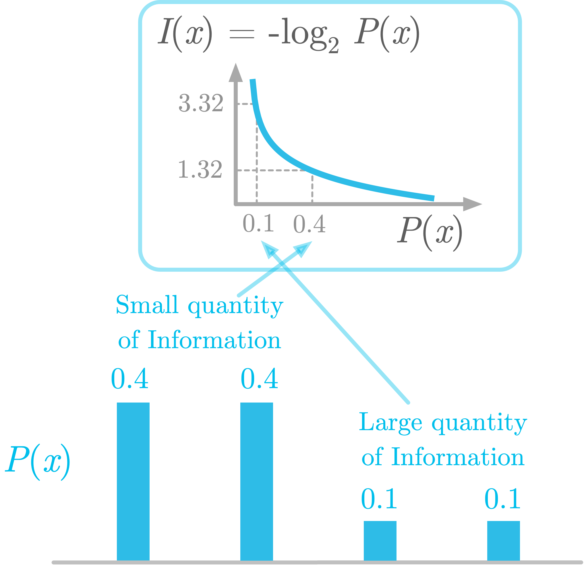
Each of these transformed probabilities is weighted by the corresponding raw probability. If an outcome occurs frequently, it will give more weight into the entropy of the distribution. This means that a low probability (like 0.1 in Figure 2) gives a large amount of information (3.32 bits) but has less influence on the final result. A larger probability (like 0.4 in Figure 2) is associated with less information (1.32 bits as shown in Figure 2) but has more weight.

Binary Entropy Function

In the example of a biased coin, you calculated the entropy of a Bernoulli process (more details about the Bernoulli distribution in Essential Math for Data Science). In this special case, the entropy is called the binary entropy function.

To characterize the binary entropy function, you’ll calculate the entropy of a biased coin described by various probability distributions (from heavily biased in favor of “tails” to heavily biased in favor of “heads”).

Let’s start by creating a function to calculate the entropy of a distribution that takes an array with the probabilities as input and returns the corresponding entropy:

def entropy(P):
    return - np.sum(P * np.log2(P))

You can also use entropy() from scipy.stats, where you can specify the base of the logarithm used to calculate the entropy. Here, I have used the base-two logarithm.

Let’s take the example of a fair coin, with a probability of 0.5 of landing ‘heads’. The distribution is thus 0.5 and 1 − 0.5 = 0.5. Let’s use the function we just defined to calculate the corresponding entropy is:

p = 0.5
entropy(np.array([p, 1 - p]))

1.0

The function calculates the sum of P * np.log2(P) over each element of the array you use as input. Using an array as input As you saw in the previous section, you can expect a lower entropy for biased coin. Let’s plot the entropy for various coin biases, from a coin landing only as ‘tails’ to a coin landing only as ‘heads’:

x_axis = np.arange(0.01, 1, 0.01)
entropy_all = []
for p in x_axis:
    entropy_all.append(entropy([p, 1 - p]))

# [...] plots the entropy

Figure 3: Entropy as a function of the probability to land “heads”.

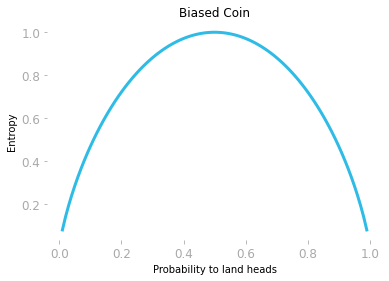
Figure 3 shows that the entropy increases until you reach the more uncertain condition: that is, when the probability of landing ‘heads’ equals the probability of landing ‘tails’.

Differential Entropy

The entropy of a continuous distribution is called differential entropy. It is an extension of the entropy for discrete distribution, but it doesn’t satisfy the same requirements. The issue is that values have probability tending to zero with continuous distributions, and encoding this would require a number of bits tending to infinity.

It is defined as:

Differential entropy can be negative. The reason is that, as you saw in Essential Math for Data Science, continuous distributions are not probabilities but probability densities, meaning that they don’t satisfy the requirements of probabilities. For instance, they are not constrained to be lower than 1. This has the consequence that p(x) can take positive values larger than 1 and log2p(x) can take positive values (leading to negative values because of the negative sign).

Cross Entropy

 
The concept of entropy can be used to compare two probability distributions: this is called the cross entropy between two distributions, which measures how much they differ.

The idea is to calculate the information associated with the probabilities of a distribution Q(x), but instead of weighting according to Q(x) as with the entropy, you weight according to the other distribution P(x). Note that you compare two distributions concerning the same random variable X.

You can also consider cross-entropy as the expected quantity of information of events drawn from P(x) when you use Q(x) to encode them.

This is mathematically expressed as:

Let’s see how it works.

Figure 4: Illustration of the cross entropy as the Shannon information of Q(x) weighted according to the distribution of P(x).

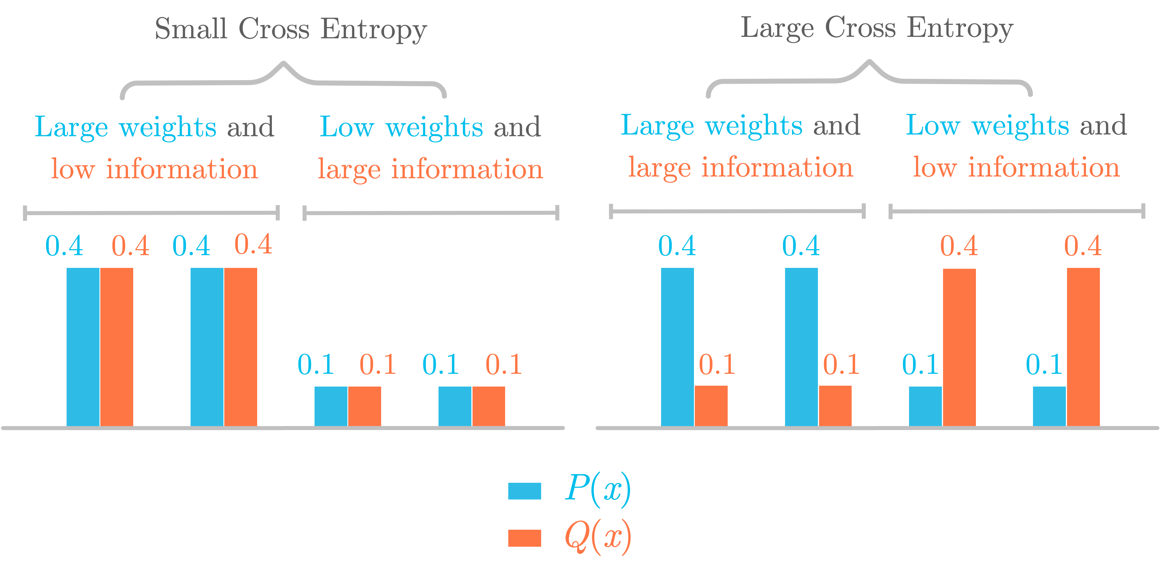
Figure 4 shows two different situations to illustrate the cross entropy. In the left, you have two identical distributions P(x) (in blue) and Q(x) (in red). Their cross entropy is equal to the entropy because the information of Q(x) is weighted according to the distribution of P(x), which is similar to Q(x).

However, in the right panel, P(x) and Q(x) are different. This results in a larger cross entropy, because probabilities associated with a large quantity of information have a small weight, while probabilities associated with a small quantity of information have large weights.

The cross entropy can’t be smaller than the entropy. Still in the right panel, you can see that, when the probability Q(x) is larger than P(x) (and thus associated with a lower amount of information), it is counterbalanced by the low weights (resulting in low weights and low information). These low weights will be compensated with larger weights in other probabilities from the distribution (resulting in large weights and large information).

Note also that both distributions P(x) and Q(x) must have the same support (that is the same set of values that the random variable can take associated with positive probabilities).

To summarize, the cross entropy is minimum when the distributions are identical. As you’ll see in 0.1.4, this property makes the cross entropy a useful metric. Note also that the result is different according to the distribution you choose as a reference: H(P,Q) ≠ H(Q,P).

Cross Entropy as a Loss Function

In machine learning, cross entropy is used as a loss function called the cross entropy loss (also called the log loss, or the logistic loss, because it is used in logistic regression).

Figure 5: Cross entropy can be used to compare the true distribution (probability of 1 for the correct class and 0 otherwise) and the distribution estimated by the model.

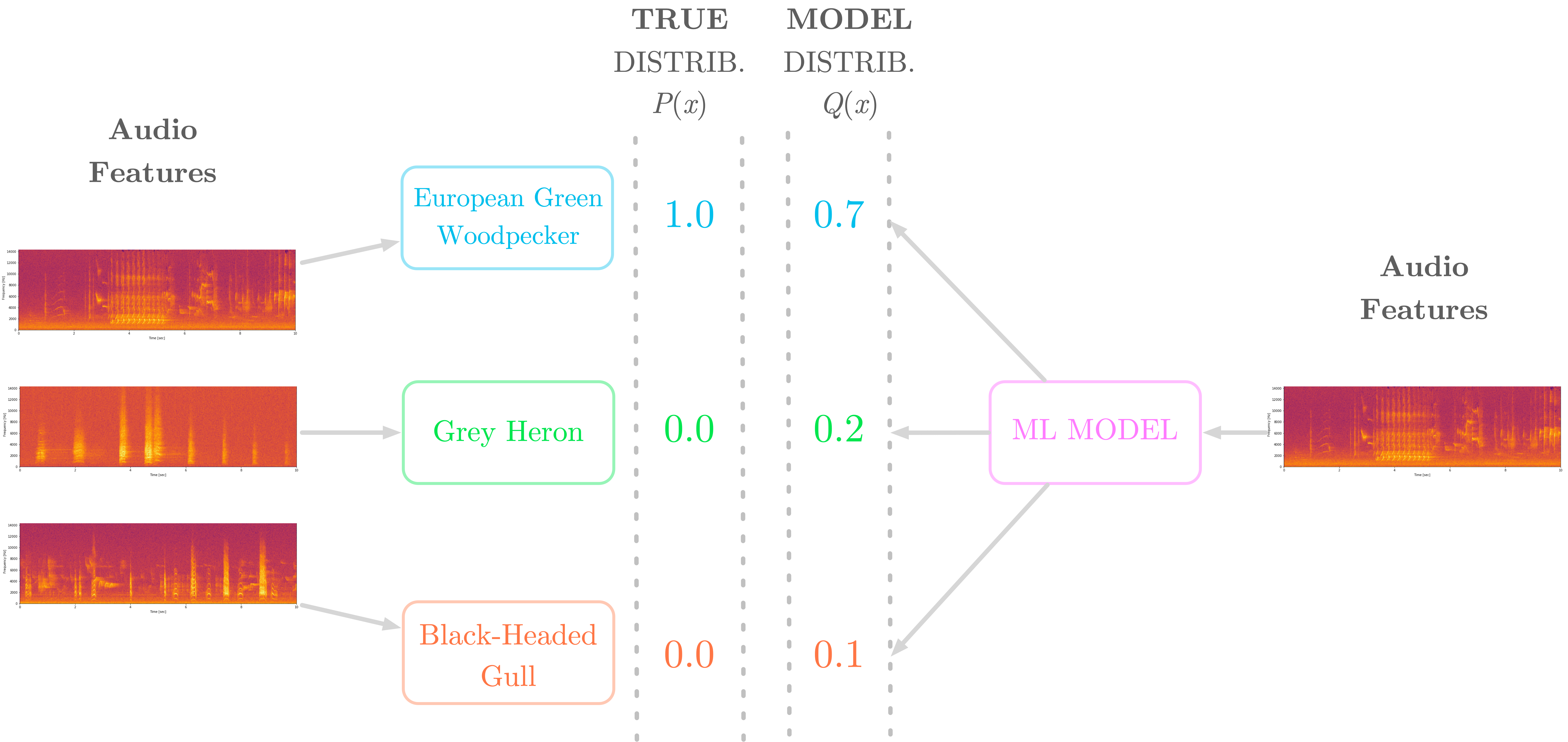
Say you want to build a model that classifies three different bird species from audio samples. As illustrated in Figure 5, the audio samples are converted in features (here spectrograms) and the possible classes (the three different birds) are one-hot encoded, that is, encoded as 1 for the correct class and 0 otherwise. Furthermore, the machine learning model outputs probabilities for each class.

To learn how to classify the birds, the model needs to compare the estimated distribution Q(x) (given by the model) and the true distribution P(x). The cross entropy loss is computed as the cross entropy between P(x) and Q(x).

Figure 5 shows that the true class corresponding the sample you consider in this example is “European Green Woodpecker”. The model outputs a probability distribution and you’ll compute the cross entropy loss associated with this estimation. Figure 6 shows both distributions.

Figure 6: Comparison of the true distribution P(x) and the estimated distribution Q(x).

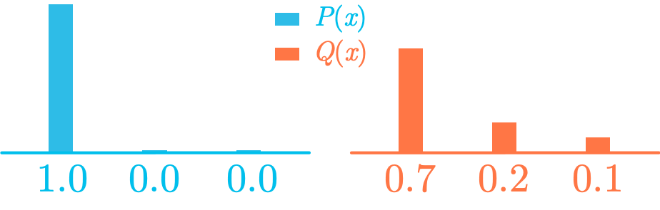
Let’s manually calculate the cross entropy between these two distributions:

The natural logarithm is used in the cross-entropy loss instead of the base-two logarithm, but the principle is the same. In addition, note the use of H(P,Q) instead of H(Q,P) because the reference is the distribution P.

Since you one-hot encoded the classes (1 for the true class and 0 otherwise), the cross entropy is simply the negative logarithm of the estimated probability for the true class.

Binary Classification: Log Loss

In machine learning, the cross entropy is widely used as a loss for binary classification: the log loss.

Since the classification is binary, the only possible outcomes are y (the true label corresponds to the first class) and 1−y (the true label corresponds to the second class). Similarly, you have the estimated probability of the first class y^ and the estimated probability of the second class 1−y^.

From the formula of the cross entropy, ∑x corresponds here to the sum over the two possible outcomes (y and 1−y). You have:

which is the formula of the log loss.

Kullback-Leibler Divergence (KL Divergence)

 
You saw that the cross entropy is a value which depends on the similarity of two distributions, with the smaller cross entropy value corresponding to identical distributions. You can use this property to calculate the divergence between two distributions: you compare their cross entropy with the situation where the distributions are identical. This divergence is called the Kullback-Leibler divergence (or simply the KL divergence), or the relative entropy.

Intuitively, the KL divergence is the supplemental amount of information associated with the encoding of the distribution Q(x) compared to the true distribution P(x). It tells you how different the two distributions are.

Mathematically, the KL divergence between two distributions P(x) and Q(x), denoted as DKL(P||Q), is expressed as the difference between the cross entropy of P(x) and Q(x) and the entropy of P(x):

Replacing with the expressions of the cross entropy and the entropy, you get:

The KL divergence is always non-negative. Since the entropy H(P) is identical to the cross entropy H(P,P), and because the smallest cross entropy is between identical distributions (H(P,P)H(P,P)), H(P,Q) is necessarily larger than H(P). In addition, the KL divergence is equal to zero when the two distributions are identical.

However, the cross entropy is not symmetrical. Comparing a distribution P(x) to a distribution Q(x) can be different than comparing a distribution Q(x) to P(x) – which implies that you can’t consider the KL divergence to be a distance.

 
Bio: Hadrien Jean is a machine learning scientist. He owns a Ph.D in cognitive science from the Ecole Normale Superieure, Paris, where he did research on auditory perception using behavioral and electrophysiological data. He previously worked in industry where he built deep learning pipelines for speech processing. At the corner of data science and environment, he works on projects about biodiversity assessement using deep learning applied to audio recordings. He also periodically creates content and teaches at Le Wagon (data science Bootcamp), and writes articles in his blog (hadrienj.github.io).

Original. Reposted with permission.

Related:

• Essential Math for Data Science: The Poisson Distribution
• Essential Math for Data Science: Probability Density and Probability Mass Functions
• Essential Math for Data Science: Integrals And Area Under The Curve