Time Series Forecasting with PyCaret Regression Module

PyCaret is an alternate low-code library that can be used to replace hundreds of lines of code with few lines only. See how to use PyCaret's Regression Module for Time Series Forecasting.

comments

By Moez Ali, Founder & Author of PyCaret

PyCaret

PyCaret is an open-source, low-code machine learning library and end-to-end model management tool built-in Python for automating machine learning workflows. It is incredibly popular for its ease of use, simplicity, and ability to build and deploy end-to-end ML prototypes quickly and efficiently.

PyCaret is an alternate low-code library that can be used to replace hundreds of lines of code with few lines only. This makes the experiment cycle exponentially fast and efficient.

PyCaret is simple and easy to use. All the operations performed in PyCaret are sequentially stored in a Pipeline that is fully automated for deployment. Whether it's imputing missing values, one-hot-encoding, transforming categorical data, feature engineering, or even hyperparameter tuning, PyCaret automates all of it. To learn more about PyCaret, watch this 1-minute video.

PyCaret — An open-source, low-code machine learning library in Python

This tutorial assumes that you have some prior knowledge and experience with PyCaret. If you haven’t used it before, no problem — you can get a quick headstart through these tutorials:

Installing PyCaret

Installing PyCaret is very easy and takes only a few minutes. We strongly recommend using a virtual environment to avoid potential conflicts with other libraries.

PyCaret’s default installation is a slim version of pycaret which only installs hard dependencies that are listed here.

# install slim version (default)
pip install pycaret# install the full version
pip install pycaret[full]

When you install the full version of pycaret, all the optional dependencies as listed here are also installed.

???? PyCaret Regression Module

PyCaret Regression Module is a supervised machine learning module used for estimating the relationships between a dependent variable (often called the ‘outcome variable’, or ‘target’) and one or more independent variables (often called ‘features’, or ‘predictors’).

The objective of regression is to predict continuous values such as sales amount, quantity, temperature, number of customers, etc. All modules in PyCaret provide many pre-processing features to prepare the data for modeling through the setup function. It has over 25 ready-to-use algorithms and several plots to analyze the performance of trained models.

???? Time Series with PyCaret Regression Module

Time series forecasting can broadly be categorized into the following categories:

Classical / Statistical Models — Moving Averages, Exponential smoothing, ARIMA, SARIMA, TBATS
Machine Learning — Linear Regression, XGBoost, Random Forest, or any ML model with reduction methods
Deep Learning — RNN, LSTM

This tutorial is focused on the second category i.e. Machine Learning.

PyCaret’s Regression module default settings are not ideal for time series data because it involves few data preparatory steps that are not valid for ordered data (data with a sequence such as time series data).

For example, the split of the dataset into train and test set is done randomly with shuffling. This wouldn’t make sense for time series data as you don’t want the recent dates to be included in the training set whereas historical dates are part of the test set.

Time-series data also requires a different kind of cross-validation since it needs to respect the order of dates. PyCaret regression module by default uses k-fold random cross-validation when evaluating models. The default cross-validation setting is not suitable for time-series data.

The following section in this tutorial will demonstrate how you can change default settings in PyCaret Regression Module easily to make it work for time series data.

???? Dataset

For the purpose of this tutorial, I have used the US airline passengers dataset. You can download the dataset from Kaggle.

# read csv file
import pandas as pd
data = pd.read_csv('AirPassengers.csv')
data['Date'] = pd.to_datetime(data['Date'])
data.head()

Sample rows

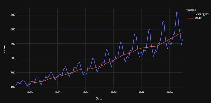
# create 12 month moving average
data['MA12'] = data['Passengers'].rolling(12).mean()# plot the data and MA
import plotly.express as px
fig = px.line(data, x="Date", y=["Passengers", "MA12"], template = 'plotly_dark')
fig.show()

US Airline Passenger Dataset Time Series Plot with Moving Average = 12

Since algorithms cannot directly deal with dates, let’s extract some simple features from dates such as month and year, and drop the original date column.

# extract month and year from dates
month = [i.month for i in data['Date']]
year = [i.year for i in data['Date']]# create a sequence of numbers
data['Series'] = np.arange(1,len(data)+1)# drop unnecessary columns and re-arrange
data.drop(['Date', 'MA12'], axis=1, inplace=True)
data = data[['Series', 'Year', 'Month', 'Passengers']] # check the head of the dataset
data.head()

Sample rows after extracting features

# split data into train-test set
train = data[data['Year'] < 1960]
test = data[data['Year'] >= 1960]# check shape
train.shape, test.shape
>>> ((132, 4), (12, 4))

I have manually split the dataset before initializing the setup . An alternate would be to pass the entire dataset to PyCaret and let it handle the split, in which case you will have to pass data_split_shuffle = False in the setup function to avoid shuffling the dataset before the split.

???? Initialize Setup

Now it’s time to initialize the setup function, where we will explicitly pass the training data, test data, and cross-validation strategy using the fold_strategy parameter.

# import the regression module
from pycaret.regression import *# initialize setup
s = setup(data = train, test_data = test, target = 'Passengers', fold_strategy = 'timeseries', numeric_features = ['Year', 'Series'], fold = 3, transform_target = True, session_id = 123)

???? Train and Evaluate all Models

best = compare_models(sort = 'MAE')

Results from compare_models

The best model based on cross-validated MAE is Least Angle Regression (MAE: 22.3). Let’s check the score on the test set.

prediction_holdout = predict_model(best);

Results from predict_model(best) function

MAE on the test set is 12% higher than the cross-validated MAE. Not so good, but we will work with it. Let’s plot the actual and predicted lines to visualize the fit.

# generate predictions on the original dataset
predictions = predict_model(best, data=data)# add a date column in the dataset
predictions['Date'] = pd.date_range(start='1949-01-01', end = '1960-12-01', freq = 'MS')# line plot
fig = px.line(predictions, x='Date', y=["Passengers", "Label"], template = 'plotly_dark')# add a vertical rectange for test-set separation
fig.add_vrect(x0="1960-01-01", x1="1960-12-01", fillcolor="grey", opacity=0.25, line_width=0)fig.show()

Actual and Predicted US airline passengers (1949–1960)

The grey backdrop towards the end is the test period (i.e. 1960). Now let’s finalize the model i.e. train the best model i.e. Least Angle Regression on the entire dataset (this time, including the test set).

final_best = finalize_model(best)

???? Create a future scoring dataset

Now that we have trained our model on the entire dataset (1949 to 1960), let’s predict five years out in the future through 1964. To use our final model to generate future predictions, we first need to create a dataset consisting of the Month, Year, Series column on the future dates.

future_dates = pd.date_range(start = '1961-01-01', end = '1965-01-01', freq = 'MS')future_df = pd.DataFrame()future_df['Month'] = [i.month for i in future_dates]
future_df['Year'] = [i.year for i in future_dates]    
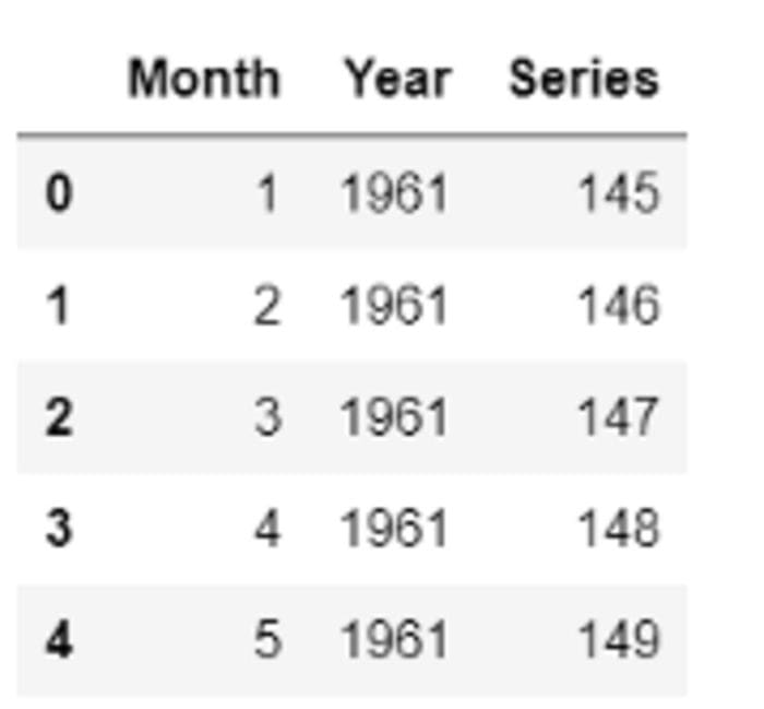
future_df['Series'] = np.arange(145,(145+len(future_dates)))future_df.head()

Sample rows from future_df

Now, let’s use the future_df to score and generate predictions.

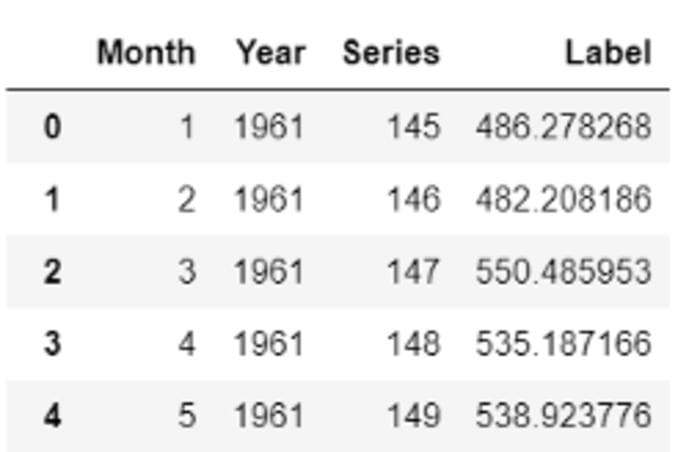
predictions_future = predict_model(final_best, data=future_df)
predictions_future.head()

Sample rows from predictions_future

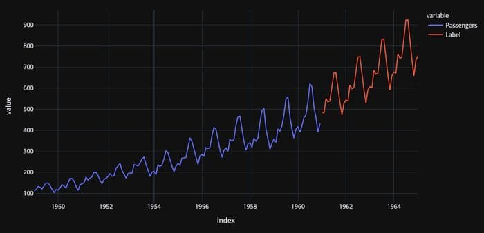
Let’s plot it.

concat_df = pd.concat([data,predictions_future], axis=0)
concat_df_i = pd.date_range(start='1949-01-01', end = '1965-01-01', freq = 'MS')
concat_df.set_index(concat_df_i, inplace=True)fig = px.line(concat_df, x=concat_df.index, y=["Passengers", "Label"], template = 'plotly_dark')
fig.show()

Actual (1949–1960) and Predicted (1961–1964) US airline passengers

Wasn’t that easy?

There is no limit to what you can achieve using this lightweight workflow automation library in Python. If you find this useful, please do not forget to give us ⭐️ on our GitHub repository.

To hear more about PyCaret follow us on LinkedIn and Youtube.

Join us on our slack channel. Invite link here.

You may also be interested in:

Build your own AutoML in Power BI using PyCaret 2.0
Deploy Machine Learning Pipeline on Azure using Docker
Deploy Machine Learning Pipeline on Google Kubernetes Engine
Deploy Machine Learning Pipeline on AWS Fargate
Build and deploy your first machine learning web app
Deploy PyCaret and Streamlit app using AWS Fargate serverless
Build and deploy machine learning web app using PyCaret and Streamlit
Deploy Machine Learning App built using Streamlit and PyCaret on GKE

Important Links

Documentation
Blog
GitHub
StackOverflow
Install PyCaret
Notebook Tutorials
Contribute in PyCaret

Want to learn about a specific module?

Click on the links below to see the documentation and working examples.

Classification
Regression
Clustering
Anomaly Detection
Natural Language Processing
Association Rule Mining

Bio: Moez Ali is a Data Scientist, and is Founder & Author of PyCaret.

Original. Reposted with permission.

Related: