A Comprehensive Guide to Ensemble Learning – Exactly What You Need to Know

Ensemble learning techniques have been proven to yield better performance on machine learning problems. We can use these techniques for regression as well as classification problems.

The final prediction from these ensembling techniques is obtained by combining results from several base models. Averaging, voting and stacking are some of the ways the results are combined to obtain a final prediction.

In this article, we will explore how ensemble learning can be used to come up with optimal machine learning models.

What is ensemble learning?

 
Ensemble learning is a combination of several machine learning models in one problem. These models are known as weak learners. The intuition is that when you combine several weak learners, they can become strong learners.

Each weak learner is fitted on the training set and provides predictions obtained. The final prediction result is computed by combining the results from all the weak learners.

Basic ensemble learning techniques

 
Let’s take a moment and look at simple ensemble learning techniques.

Max voting

In classification, the prediction from each model is a vote. In max voting, the final prediction comes from the prediction with the most votes.

Let’s take an example where you have three classifiers with the following predictions:

• classifier 1 – class A
• classifier 2 – class B
• classifier 3 – class B

The final prediction here would be class B since it has the most votes.

Averaging

In averaging, the final output is an average of all predictions. This goes for regression problems. For example, in random forest regression, the final result is the average of the predictions from individual decision trees.

Let’s take an example of three regression models that predict the price of a commodity as follows:

• regressor 1 – 200
• regressor 2 – 300
• regressor 3 – 400

The final prediction would be the average of 200, 300, and 400.

Weighted average

In weighted averaging, the base model with higher predictive power is more important. In the price prediction example, each of the regressors would be assigned a weight.

The sum of the weights would equal one. Let’s say that the regressors are given weights of 0.35, 0.45, and 0.2 respectively. The final model prediction can be computed as follows:

0.35 * 200 + 0.45*300 + 0.2*400 = 285

Advanced ensemble learning techniques

 
Above are simple techniques, now let’s take a look at advanced techniques for ensemble learning.

Stacking

 
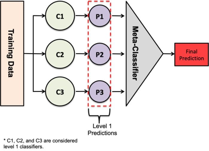
Stacking is the process of combining various estimators in order to reduce their biases. Predictions from each estimator are stacked together and used as input to a final estimator (usually called a meta-model) that computes the final prediction. Training of the final estimator happens via cross-validation.

Stacking can be done for both regression and classification problems.

Source

Stacking can be considered to happen in the following steps:

1. Split the data into a training and validation set,
2. Divide the training set into K folds, for example 10,
3. Train a base model (say SVM) on 9 folds and make predictions on the 10th fold,
4. Repeat until you have a prediction for each fold,
5. Fit the base model on the whole training set,
6. Use the model to make predictions on the test set,
7. Repeat step 3 – 6 for other base models (for example decision trees),
8. Use predictions from the test set as features to a new model – the meta-model,
9. Make final predictions on the test set using the meta model.

With regression problems, the values passed to the meta-model are numeric. With classification problems, they’re probabilities or class labels.

Blending

 
Blending is similar to stacking, but uses a holdout set from the training set to make predictions. So, predictions are done on the holdout set only. The predictions and holdout set are used to build a final model that makes predictions on the test set.

You can think of blending as a type of stacking, where the meta-model is trained on predictions made by the base model on the hold-out validation set.

You can consider the blending process to be:

• Split the data into a test and validation set,
• Fit base models on the validation set,
• Make predictions on the validation and test set,
• Use the validation set and its predictions to build a final model,
• Make final predictions using this model.

The concept of blending was made popular by the Netflix Prize competition. The winning team used a blended solution to achieve a 10-fold performance improvement on Netflix’s movie recommendation algorithm.

According to this Kaggle ensembling guide:

“Blending is a word introduced by the Netflix winners. It’s very close to stacked generalization, but a bit simpler and less risk of an information leak. Some researchers use “stacked ensembling” and “blending” interchangeably.

With blending, instead of creating out-of-fold predictions for the train set, you create a small holdout set of say 10% of the train set. The stacker model then trains on this holdout set only.”

Blending vs stacking

 
Blending is simpler than stacking and prevents leakage of information in the model. The generalizers and the stackers use different datasets.  However, blending uses less data and may lead to overfitting.

Cross-validation is more solid on stacking than blending. It’s calculated over more folds, compared to using a small hold-out dataset in blending.

Bagging

 
Bagging takes random samples of data, builds learning algorithms, and uses the mean to find bagging probabilities. It’s also called bootstrap aggregating. Bagging aggregates the results from several models in order to obtain a generalized result.

The method involves:

• Creating multiple subsets from the original dataset with replacement,
• Building a base model for each of the subsets,
• Running all the models in parallel,
• Combining predictions from all models to obtain final predictions.

Boosting

 
Boosting is a machine learning ensemble technique that reduces bias and variance by converting weak learners into strong learners. The weak learners are applied to the dataset in a sequential manner. The first step is building an initial model and fitting it into the training set.

A second model that tries to fix the errors generated by the first model is then fitted. Here’s what the entire process looks like:

• Create a subset from the original data,
• Build an initial model with this data,
• Run predictions on the whole data set,
• Calculate the error using the predictions and the actual values,
• Assign more weight to the incorrect predictions,
• Create another model that attempts to fix errors from the last model,
• Run predictions on the entire dataset with the new model,
• Create several models with each model aiming at correcting the errors generated by the previous one,
• Obtain the final model by weighting the mean of all the models.

Libraries for ensemble learning

 
With that introduction out of the way, let’s talk about libraries that you can use for ensembling. Broadly speaking, there are two categories:

• Bagging algorithms,
• Boosting algorithms.

Bagging algorithms

 
Bagging algorithms are based on the bagging technique described above. Let’s take a look at a couple of them.

Bagging meta-estimator

Scikit-learn lets us implement a `BaggingClassifier` and a `BaggingRegressor`. The bagging meta-estimator fits each base model on random subsets of the original dataset. It then computes the final prediction by aggregating individual base model predictions. Aggregation is done by voting or averaging. The method reduces the variance of estimators by introducing randomization in their construction process.

There are several flavors of bagging:

• Drawing random subsets of the data as random subsets of the samples is referred to as pasting. 
• The algorithm is referred to as bagging when the samples are drawn with replacement.
• If random data subsets are taken as random subsets of the feature, the algorithm is referred to as Random Subspaces.
• When you create base estimators from subsets of both samples and features, it’s Random Patches.

Let’s take a look at how you can create a bagging estimator using Scikit-learn.

This takes a few steps:

• Import the `BaggingClassifier`,
• Import a base estimator – a decision tree classifier,
• Create an instance of the `BaggingClassifier`.

from sklearn.ensemble import BaggingClassifier
from sklearn.tree import DecisionTreeClassifier
bagging = BaggingClassifier(base_estimator=DecisionTreeClassifier(),n_estimators=10, max_samples=0.5, max_features=0.5)

The bagging classifier takes several arguments:

• The base estimator – here, a decision tree classifier,
• The number of estimators you want in the ensemble,
• `max_samples` to define the number of samples that will be drawn from the training set for each base estimator ,
• `max_features` to dictate the number of features that will be used to train each base estimator.

Next, you can fit this classifier on the training set and score it.

bagging.fit(X_train, y_train)
bagging.score(X_test,y_test)

The process will be the same for regression problems, the only difference being that you will work with regression estimators.

from sklearn.ensemble import BaggingRegressor
bagging = BaggingRegressor(DecisionTreeRegressor())
bagging.fit(X_train, y_train)
model.score(X_test,y_test)

Forests of randomized trees

A Random Forest® is an ensemble of random decision trees. Each decision tree is created from a different sample of the dataset. The samples are drawn with replacement. Every tree produces its own prediction.

In regression, these results are averaged to obtain the final result.

In classification, the final result can be obtained as the class with the most votes.

The averaging and voting improves the accuracy of the model by preventing overfitting.

In Scikit-learn a forest of randomized trees can be implemented via `RandomForestClassifier` and the `ExtraTreesClassifier`. Similar estimators are available for regression problems.

from sklearn.ensemble import RandomForestClassifier
from sklearn.ensemble import ExtraTreesClassifier
clf = RandomForestClassifier(n_estimators=10, max_depth=None,  min_samples_split=2, random_state=0)
clf.fit(X_train, y_train)
clf.score(X_test,y_test)

clf = ExtraTreesClassifier(n_estimators=10, max_depth=None, min_samples_split=2, random_state=0)
clf.fit(X_train, y_train)
clf.score(X_test,y_test)

Boosting algorithms

 
These algorithms are based on the boosting framework described earlier. Let’s look at a few of them.

AdaBoost

AdaBoost works by fitting a sequence of weak learners. It gives incorrect predictions more weight in subsequent iterations, and less weight to correct predictions. This forces the algorithm to focus on observations that are harder to predict. The final prediction comes from weighing the majority vote or sum.

AdaBoost can be used for both regression and classification problems. Let’s take a moment and look at how you can apply the algorithm to a classification problem using Scikit-learn.

We use the `AdaBoostClassifier`. `n_estimators` dictates the number of weak learners in the ensemble. The contribution of each weak learner to the final combination is controlled by the `learning_rate`.

By default, decision trees are used as base estimators. In order to obtain better results, the parameters of the decision tree can be tuned. You can also tune the number of base estimators.

from sklearn.ensemble import AdaBoostClassifier
model = AdaBoostClassifier(n_estimators=100)
model.fit(X_train, y_train)
model.score(X_test,y_test)

Gradient tree boosting

Gradient tree boosting also combines a set of weak learners to form a strong learner. There are three main items to note, as far as gradient boosting trees are concerned:

• a differential loss function has to be used,
• decision trees are used as weak learners,
• it’s an additive model, so trees are added one after the other. Gradient descent is used to minimize the loss when adding subsequent trees.

You can use Scikit-learn to build a model based on gradient tree boosting.

from sklearn.ensemble import GradientBoostingClassifier
model = GradientBoostingClassifier(n_estimators=100, learning_rate=1.0, max_depth=1, random_state=0)
model.fit(X_train, y_train)
model.score(X_test,y_test)

eXtreme Gradient Boosting

eXtreme Gradient Boosting, popularly known as XGoost, is a top gradient boosting framework. It’s based on an ensemble of weak decision trees. It can do parallel computations on a single computer.

The algorithm uses regression trees for the base learner. It also has cross-validation built-in. Developers love it for its accuracy, efficiency, and feasibility.

import xgboost as xgb
params = {"objective":"binary:logistic",'colsample_bytree': 0.3,'learning_rate': 0.1,
                'max_depth': 5, 'alpha': 10}
model = xgb.XGBClassifier(**params)
model.fit(X_train, y_train)
model.fit(X_train, y_train)
model.score(X_test,y_test)

LightGBM

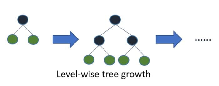
LightGBM is a gradient boosting algorithm based on tree learning. Unlike other tree-based algorithms that use depth-wise growth, LightGBM uses leaf-wise tree growth. Leaf-wise growth algorithms tend to converge faster than dep-wise-based algorithms.

Source

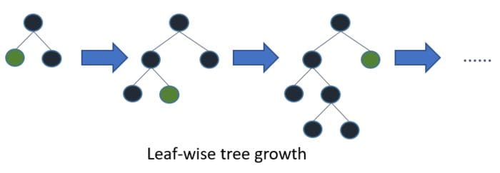Source

Source

LightGBM can be used for both regression and classification problems by setting the appropriate objective.

Here’s how you can apply LightGBM to a binary classification problem.

import lightgbm as lgb
lgb_train = lgb.Dataset(X_train, y_train)
lgb_eval = lgb.Dataset(X_test, y_test, reference=lgb_train)
params = {'boosting_type': 'gbdt',
              'objective': 'binary',
              'num_leaves': 40,
              'learning_rate': 0.1,
              'feature_fraction': 0.9
              }
gbm = lgb.train(params,
    lgb_train,
    num_boost_round=200,
    valid_sets=[lgb_train, lgb_eval],
    valid_names=['train','valid'],
   )

CatBoost

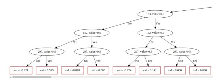
CatBoost is a depth-wise gradient boosting library developed by Yandex. It grows a balanced tree using oblivion decision trees. As you can see in the image below, the same features are used when making left and right splits at each level.

Source

Researchers need Catboost for the following reasons:

• The ability to handle categorical features natively,
• Models can be trained on several GPUs,
• It reduces parameter tuning time by providing great results with default parameters,
• Models can be exported to Core ML for on-device inference (iOS),
• It handles missing values internally,
• It can be used for both regression and classification problems.

Here’s how you can apply CatBoost to a classification problem.

from catboost import CatBoostClassifier
cat = CatBoostClassifier()
cat.fit(X_train,y_train,verbose=False, plot=True

Libraries that help you do stacking on base models

 
When stacking, the output of individual models is stacked and a final estimator used to compute the final prediction. The estimators are fitted on the whole training set. The final estimator is trained on the cross-validated predictions of the base estimators.

Scikit-learn can be used to stack estimators. Let’s take a look at how you can stack estimators for a classification problem.

First, you need to set up the base estimator that you want to use.

estimators = [
  ('knn', KNeighborsClassifier()),
   ('rf', RandomForestClassifier(n_estimators=10, random_state=42)),
   ('svr', LinearSVC(random_state=42))
]

Next, instantiate the stacking classifier. Its parameters include:

• The estimators defined above,
• The final estimator that you’d like to use. The logistic regression estimator is used by default,
• `cv` the cross-validation generator. Uses 5 k-fold cross-validation by default,
• `stack_method` to dictate the method to be applied to each estimator. If `auto`, it will try `predict_proba`, `decision_function` or `predict`’ in that order.

from sklearn.ensemble import StackingClassifier
clf = StackingClassifier(
 estimators=estimators, final_estimator=LogisticRegression()
 )

After that, you can fit the data to the training set and score it on the test set.

clf.fit(X_train, y_train)
clf.score(X_test,y_test)

Scikit-learn also lets you implement a voting estimator. It uses the majority vote or the average of the probabilities from the base estimators to make the final prediction.

This can be implemented using the  `VotingClassifier` for classification problems and the `VotingRegressor` for regression problems. Just like stacking, you will first have to define a set of base estimators.

Let’s look at how you can implement it for classification problems. The `VotingClassifier` lets you select the voting type:

• `soft` means that the average of the probabilities will be used to compute the final result,
• `hard` notifies the classifier to use the predicted classes for majority voting.

from sklearn.ensemble import VotingClassifier
voting = VotingClassifier(
    estimators=estimators,
    voting='soft')

The voting regressor uses several estimators and returns the final result as the average of predicted values.

Stacking with Mlxtend

 
You can also perform stacking using Mlxtend’s `StackingCVClassifier`. The first step is to define a list of base estimators, and then pass the estimators to the classifier.

You also have to define the final model that will be used to aggregate the predictions. In this case, it’s the logistic regression model.

knn = KNeighborsClassifier(n_neighbors=1)
rf = RandomForestClassifier(random_state=1)
gnb = GaussianNB()
lr = LogisticRegression()
estimators = [knn,gnb,rf,lr]
stack = StackingCVClassifier(classifiers = estimators,
                            shuffle = False,
use_probas = True,
cv = 5, 
meta_classifier = LogisticRegression())

When to use ensemble learning

 
You can employ ensemble learning techniques when you want to improve the performance of machine learning models. For example to increase the accuracy of classification models or to reduce the mean absolute error for regression models. Ensembling also results in a more stable model.

When your model is overfitting on the training set, you can also employ ensembling learning methods to create a more complex model. The models in the ensemble would then improve performance on the dataset by combining their predictions.

When ensemble learning works best

 
Ensemble learning works best when the base models are not correlated. For instance, you can train different models such as linear models, decision trees, and neural nets on different datasets or features. The less correlated the base models, the better.

The idea behind using uncorrelated models is that each may be solving a weakness of the other. They also have different strengths which, when combined, will result in a well-performing estimator. For example, creating an ensemble of just tree-based models may not be as effective as combining tree-type algorithms with other types of algorithms.

Final thoughts

 
In this article, we explored how to use ensemble learning to improve the performance of machine learning models. We’ve also gone through various tools and techniques that you can use for ensembling. Your machine learning repertoire has hopefully grown.

Happy ensembling!

Resources

• Kaggle ensembling guide
• Scikit-learn ensembling guide 
• Notebook used in the article

 
Bio: Derrick Mwiti is a data scientist who has a great passion for sharing knowledge. He is an avid contributor to the data science community via blogs such as Heartbeat, Towards Data Science, Datacamp, Neptune AI, KDnuggets just to mention a few. His content has been viewed over a million times on the internet. Derrick is also an author and online instructor. He also trains and works with various institutions to implement data science solutions as well as to upskill their staff. You might want to check his Complete Data Science & Machine Learning Bootcamp in Python course.

Original. Reposted with permission.

Related:

• XGBoost: What it is, and when to use it
• Gradient Boosted Decision Trees – A Conceptual Explanation
• The Best Machine Learning Frameworks & Extensions for Scikit-learn