XGBoost Explained: DIY XGBoost Library in Less Than 200 Lines of Python

Understand how XGBoost work with a simple 200 lines codes that implement gradient boosting for decision trees.

By Guillaume Saupin, CTO at Verteego

XGBoost is probably one of the most widely used libraries in data science. Many data scientists around the world are using it. It’s a very versatile algorithm that can be use to perform classification, regression as well as confidence intervals as shown in this article. But how many really understand its underlying principles?

You might think that a Machine Learning algorithm that performs as well as XGBoost might be using very complex and advanced mathematics. You probably imagine that it’s a masterpiece of software engineering.

And you’re partly right. The XGBoost library is a pretty complex one, but if you consider only the mathematical formulation of gradient boosting applied to decision trees, it’s not that complicated.

You will see below in detail how to train decision trees for regression using the gradient boosting method with less than 200 lines of code.

Decision Tree

Before getting into the mathematical details, let’s refresh our memory regarding decision trees. The principle is fairly simple: associate a value to a given set of features traversing a binary tree. Each node of the binary tree is attached to a condition; leaves contain values.

If the condition is true, we continue the traversal using the left node, if not, we use the right one. Once a leaf is reached, we have our prediction.

As often, a picture is worth a thousand words:

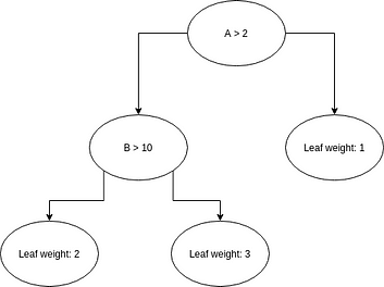
A three-level decision tree. Image by the author.

The condition attached to a node can be regarded as a decision, hence the name Decision Tree.

This kind of structure is pretty old in the history of computer science and has been used for decades with success. A basic implementation is given by the following lines:

Stacking multiple trees

Even though Decision Trees have been used with some success in a number of applications, like expert systems (before the AI winter) it remains a very basic model that cannot handle the complexity usually encountered in real-world data.

We usually refer to this kind of estimators as weak models.

To overcome this limitation, the idea emerged in the nineties to combine multiple weak models to create a strong model: ensemble learning.

This method can be applied to any kind of model, but as Decision Trees are simple, fast, generic and easily interpretable models, they are commonly used.

Various strategies can be deployed to combine models. We can for instance use a weighted sum of each model prediction. Or even better, use a Bayesian approach to combine them based on learning.

XGBoost and all boosting methods use another approach: each new model tries to compensate for the errors of the previous one.

Optimizing decision trees

As we have seen above, making predictions using a decision tree is straightforward. The job is hardly more complicated when using ensemble learning: all we have to do is sum contributions of each model.

What’s really complicated is building the tree itself! How can we find the best condition to apply at each node of our training dataset? This is where math helps us. A full derivation can be found in the XGBoost documentation. Here, we will focus only on the formulas of interest for this article.

As always in machine learning, we want to set our model parameters so that our model’s predictions on the training set minimize a given objective:

Objective formula. Formula by the author.

Please note that this objective is made of two terms:

One to measure the error made by the prediction. It’s the famous loss function l(y, y_hat).
The other, omega, to control model complexity.

As stated in the XGBoost documentation, complexity is a very important part of the objective that allows us to tune the bias/variance trade-off. Many different functions can be used to define this regularization term. XGBoost use:

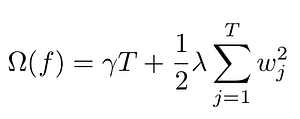
Regularization term. Formula by the author.

Here T is the total number of leaves, whereas w_j are the weights attached to each leaf. This means that a large weight and a large number of leaves will be penalized.

As the error is often a complex, non-linear function, we linearized it using second-order Taylor expansion:

Second-order expansion of the loss. Formula by the author.

where:

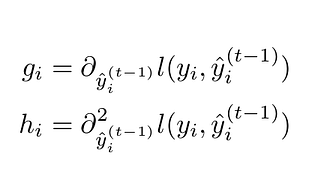
Gaussian and hessian formulas. Formula by the author.

The linearization is computed with respect to the prediction term, as we want to estimate how the error changes when the prediction changes. Linearization is essential, as it will ease the minimization of the error.

What we want to achieve with gradient boosting, is to find the optimal delta_y_i that will minimize the loss function, i.e. we want to find how to modify the existing tree so that the modification improves the prediction.

When dealing with tree models, there are two kinds of parameters to consider:

The ones defining the tree in itself: the condition for each node, the depth of the tree
The values attached to each leaf of the tree. These values are the predictions themselves.

Exploring every tree configurations would be too complex, therefore gradient tree boosting methods only consider splitting one node into two leaves. This means that we have to optimize three parameters:

The splitting value: on which condition do we split data
The value attached to the left leaf
The value attached to the right leaf

In the XGBoost documentation, the best value for a leaf j with respect to the objective is given by:

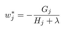
Optimal leaf value with respect to objective. Formula by the author.

where G_j is the sum of the gradient of the training points attached to the node j, and H_j is the sum of the hessian of the training points attached to the node j.

The reduction in the objective function obtained with this optimal param is:

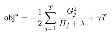
Objective improvement when using optimal weight. Formula by the author.

Choosing the right split value is done using brut force: we compute the improvement for each split value, and we keep the best one.

We now have all the required mathematical information to boost an initial tree performance with respect to a given objective by adding new leaves.

Before doing it concretely, let’s take some time to understand what these formulas mean.

Grokking gradient boosting

Let’s try to get some insight on how weight is computed, and what G_j and H_i equal to. As they are respectively the gradient and hessian of the loss function with respect to the prediction, we have to pick a loss function.

We will focus on the squared error, which is commonly used and is the default objective for XGBoost:

Squared error loss function. Formula by the author

It’s a pretty simple formula, whose gradient is:

The gradient of the loss function. Formula by the author.

and hessian:

Hessian of the loss function. Formula by the author.

Hence, if we remember the formulas for the optimal weight that maximize error reduction:

Optimal leaf value with respect to the objective. Formula by the author.

We realize that the optimal weight, i.e. the value that we add to the previous prediction is the opposite of the average error between the previous prediction and the real value (when regularization is disabled, i.e. lambda = 0). Using the squared loss to train Decision Trees with gradient boosting just boils down to updating the prediction with the average error in each new node.

We also see that lambda has the expected effect, that is ensuring that weights are not too large, as weight is inversely proportional to lambda.

Training decision trees

Now comes the easy part. Let’s say that we have an existing decision tree that ensures predictions with a given error. We want to reduce the error and improve the attached objective by splitting one node.

The algorithm to do so is pretty straightforward:

Pick a feature of interest
Order data points attached to the current node using values of the selected feature
pick a possible split value
Put data points below this split value in the right node, and the one above in the left node
compute objective reduction for the parent node, the right node and the left one
If the sum of the objective reduction for left and right nodes is greater than the one of the parent node, keep the split value as the best one
Iterate for each split value
Use the best split value if any, and add the two new nodes
If no splitting improved the objective, don’t add child nodes.

The resulting code creates a DecisionTree class, that is configured by an objective, a number of estimators, i.e. the number of trees, and a max depth.

As promised the code takes less than 200 lines:

The core of the training is coded in the function _find_best_split. It essentially follows the steps detailed above.

Note that to support any kind of objective, without the pain of manually calculating the gradient and the hessian, we use automatic differentiation and the jax library to automate computations.

Initially, we start with a tree with only one node whose leaf value leaf is zero. As we have mimic XGBoost, we also use a base score, that we set to be the mean of the value to predict.

Also, note that at line 126 we stop tree building if we reach the max depth defined when initializing the tree. We could have used other conditions like a minimum number of sample for each leaf or a minimum value for the new weight.

Another very important point is the choice of the feature used for the splitting. Here, for the sake of simplicity, features are selected randomly, but we could have been using smarter strategies, like using the feature having the greatest variance.

Conclusion

In this article, we have seen how gradient boosting works to train decision trees. To further improve our understanding, we have written the minimal set of lines required to train an ensemble of decision trees and use them for prediction.

Having a deep understanding of the algorithms we use for machine learning is absolutely critical. It not only helps us building better models but more importantly allows us to bend these models to our needs.

For instance, in the case of gradient boosting, playing with loss functions is an excellent way to increase precision when predicting.

Bio: Guillaume Saupin is CTO at Verteego.

Original. Reposted with permission.

Related: