Image by Author

The imbalanced dataset is a problem in data science. The problem happens because imbalance often leads to modeling performance issues. To mitigate the imbalance problem, we can use the oversampling method. Oversampling is the minority resampling data to balance out the data. 

There are many ways to oversample, and of them is by using SMOTE1. Let’s explore many SMOTE implementations to learn further about oversampling techniques.

SMOTE Variations

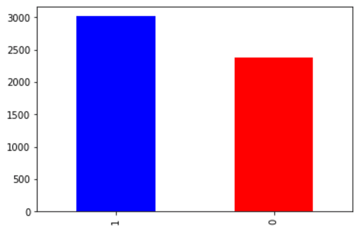
Before we continue further, we will use the churn dataset from Kaggle2 to represent the imbalanced dataset. The dataset target is the  ‘exited’ variable, and we would see how the SMOTE would oversample the data based on the minority target.

import pandas as pd

df = pd.read_csv('churn.csv')
df['Exited'].value_counts().plot(kind = 'bar', color = ['blue', 'red'])

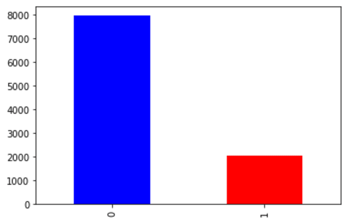
We can see that our churn dataset is faced with an imbalance problem. Let’s try the SMOTE to oversample the data.

1. SMOTE

SMOTE is commonly used to oversample continuous data for ML problems by developing artificial or synthetic data. We are using continuous data because the model for developing the sample only accepts continuous data1.

For our example, we would use two continuous variables from the dataset example; ‘EstimatedSalary’ and ‘Age’. Let’s see how both variables spread compared to the data target.

import seaborn as sns
sns.scatterplot(data =df, x ='EstimatedSalary', y = 'Age', hue = 'Exited')

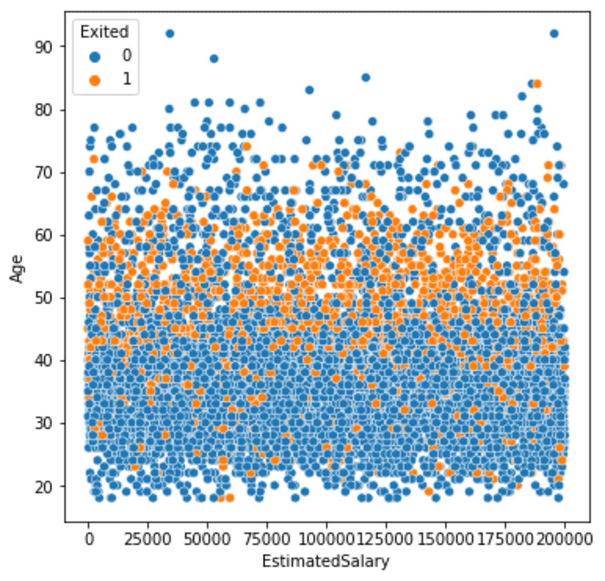
We can see the minority class mostly spread on the middle part of the plot. Let’s try to oversample the data with SMOTE and see how the differences were made. To facilitate the SMOTE oversampling, we would use the imblearn Python package.

pip install imblearn

With imblearn, we would oversample our churn data. 

from imblearn.over_sampling import SMOTE
smote = SMOTE(random_state = 42)

X, y = smote.fit_resample(df[['EstimatedSalary', 'Age']], df['Exited'])
df_smote = pd.DataFrame(X, columns = ['EstimatedSalary', 'Age'])
df_smote['Exited'] = y

Imblearn package is based on the scikit-learn API, which was easy to use. In the example above, we have oversampled the dataset with SMOTE. Let’s see the ‘Exited’ variable distribution.

df_smote['Exited'].value_counts().plot(kind = 'bar', color = ['blue', 'red'])

As we can see from the output above, the target variable now has similar proportions. Let’s see how the continuous variable spread with the new SMOTE oversampled data.

import matplotlib.pyplot as plt

sns.scatterplot(data = df_smote, x ='EstimatedSalary', y = 'Age', hue = 'Exited')
plt.title('SMOTE')

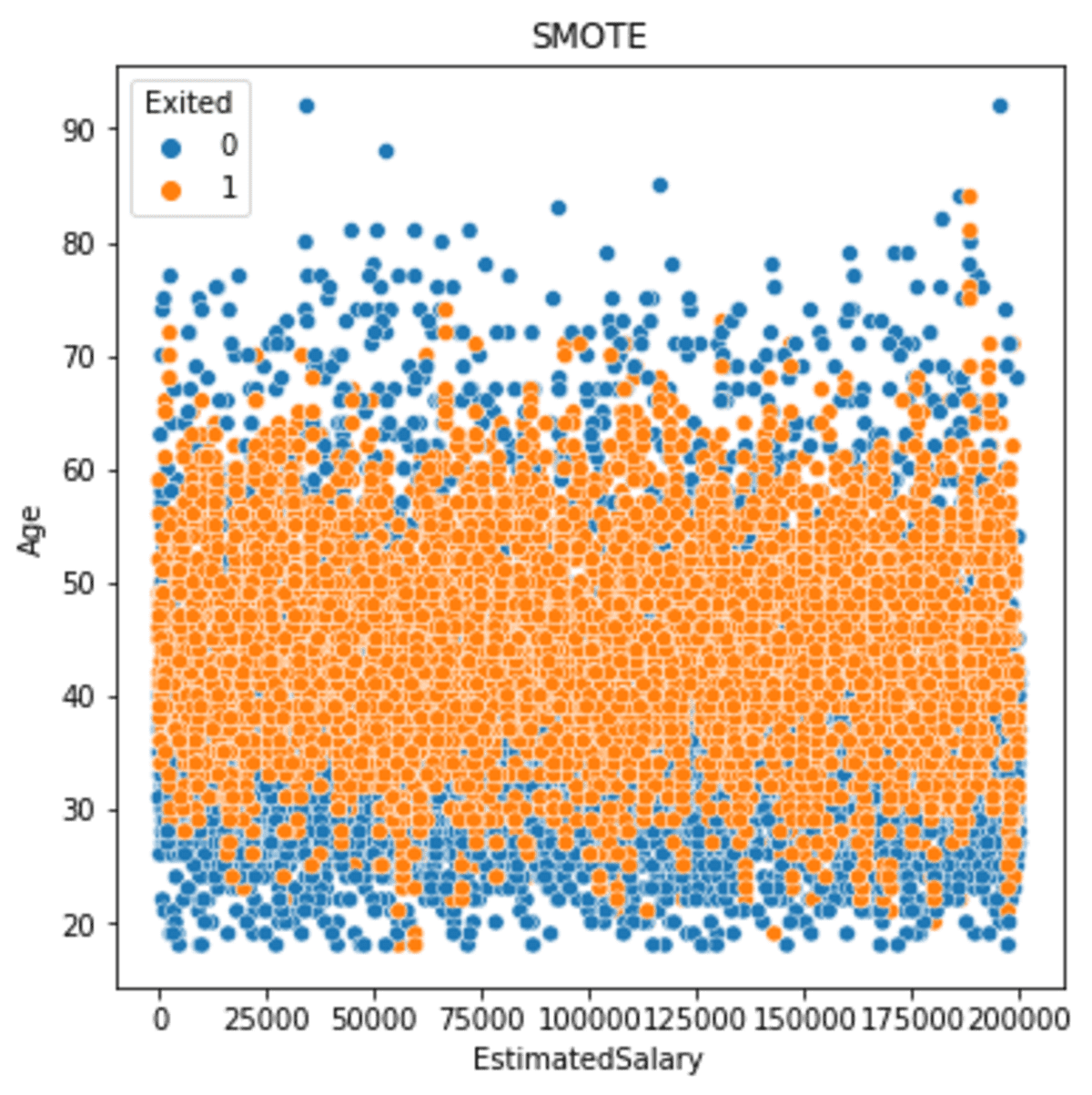
The above image shows the minority data is now spread more than before we oversample the data. If we see the output in more detail, we can see that the minority data spread is still close to the core and has spread wider than before.  This happens because the sample was based on the neighbor model, which estimated the sample based on the nearest neighbor.

2. SMOTE-NC

SMOTE-NC is SMOTE for the categorical data. As I mentioned above, SMOTE only works for continuous data.

Why don’t we just encode the categorical variable into the continuous variable?

The problem is the SMOTE creates a sample based on the nearest neighbor. If you encode the categorical data, say the ‘HasCrCard’ variable, which contains classes 0 and 1, the sample result could be 0.8 or 0.34, and so on. 

From the data standpoint, it doesn’t make sense. That is why we could use SMOTE-NC to ensure that the categorical data oversampling would make sense. 

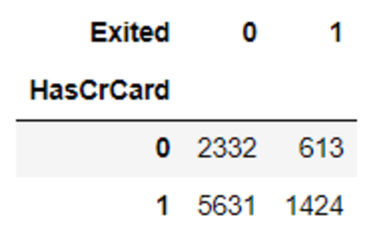
Let’s try with example data. For this specific sample, we would use the variables ‘HasCrCard’ and ‘Age’. First, I want to show the initial ‘HasCrCard’ variable spread.

pd.crosstab(df['HasCrCard'], df['Exited'])

Then let’s see the differences after the oversampling process with SMOTE-NC.

from imblearn.over_sampling import SMOTENC

smotenc = SMOTENC([1],random_state = 42)
X_os_nc, y_os_nc = smotenc.fit_resample(df[['Age', 'HasCrCard']], df['Exited'])

Notice in the above code, the categorical variable position is based on the variable position in the DataFrame. 

Let’s see how the ‘HasCrCard’ spread after the oversampling.

pd.crosstab(X_os_nc['HasCrCard'], y_os_nc)

See that the data oversampling almost have the same proportions. You could try with another categorical variable to see how SMOTE-NC works.

3. Borderline-SMOTE

Borderline-SMOTE is a SMOTE that is based on the classifier borderline. Borderline-SMOTE would oversample the data that was close to the classifier borderline. This is because the closer the sample from the borderline is expected to be prone to misclassified and thus more important to oversampled.3

There are two kinds of Borderline-SMOTE; Borderline-SMOTE1 and Borderline-SMOTE2. The differences are Borderline-SMOTE1 would oversample both classes that are close to the borderline. In comparison, Borderline-SMOTE2 would only oversample the minority class.

Let’s try the Borderline-SMOTE with a dataset example.

from imblearn.over_sampling import BorderlineSMOTE
bsmote = BorderlineSMOTE(random_state = 42, kind = 'borderline-1')
X_bd, y_bd = bsmote.fit_resample(df[['EstimatedSalary', 'Age']], df['Exited'])
df_bd = pd.DataFrame(X_bd, columns = ['EstimatedSalary', 'Age'])
df_bd['Exited'] = y_bd

Let’s see how the spread after we initiate the Borderline-SMOTE.

sns.scatterplot(data = df_bd, x ='EstimatedSalary', y = 'Age', hue = 'Exited')
plt.title('Borderline-SMOTE')

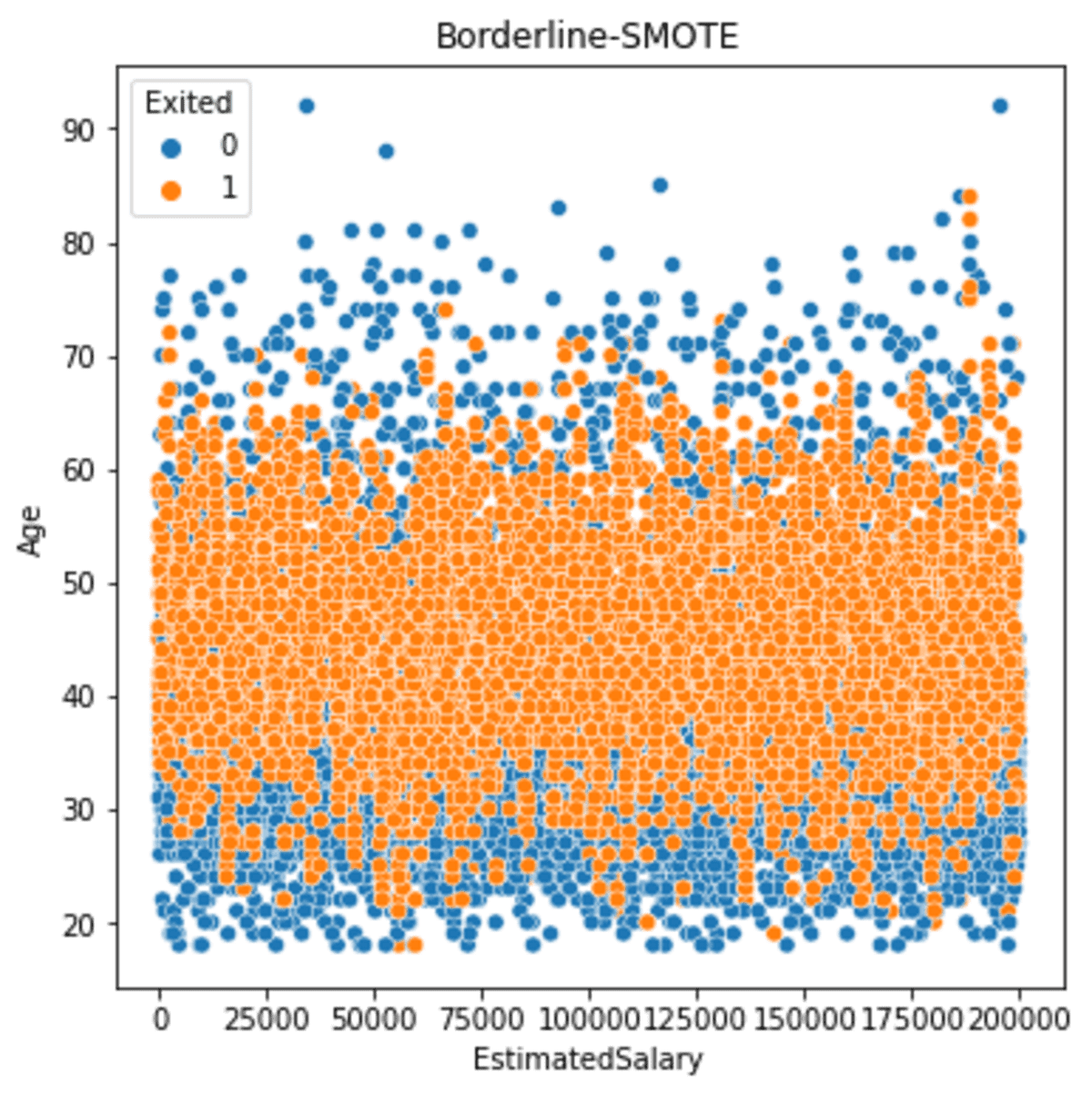
If we see the result above, the output is similar to the SMOTE output, but Borderline-SMOTE oversampling results slightly closer to the borderline. 

4. SMOTE-Tomek

SMOTE-Tomek uses a combination of both SMOTE and the undersampling Tomek link. Tomek link is a cleaning data way to remove the majority class that was overlapping with the minority class4. 

Let’s try SMOTE-TOMEK to the sample dataset.

from imblearn.combine import SMOTETomek

s_tomek = SMOTETomek(random_state = 42)
X_st, y_st = s_tomek.fit_resample(df[['EstimatedSalary', 'Age']], df['Exited'])
df_st = pd.DataFrame(X_st, columns = ['EstimatedSalary', 'Age'])
df_st['Exited'] = y_st

Let’s take a look at the target variable result after we use SMOTE-Tomek.

df_st['Exited'].value_counts().plot(kind = 'bar', color = ['blue', 'red'])

The 'Exited' class 0 number is now around 6000 compared to the original dataset, which is close to 8000. This happens because SMOTE-Tomek undersampled the class 0 while oversampling the minority class.

Let’s see how the data spread after we oversample the data with SMOTE-Tomek.

sns.scatterplot(data = df_st, x ='EstimatedSalary', y = 'Age', hue = 'Exited')
plt.title('SMOTE-Tomek')

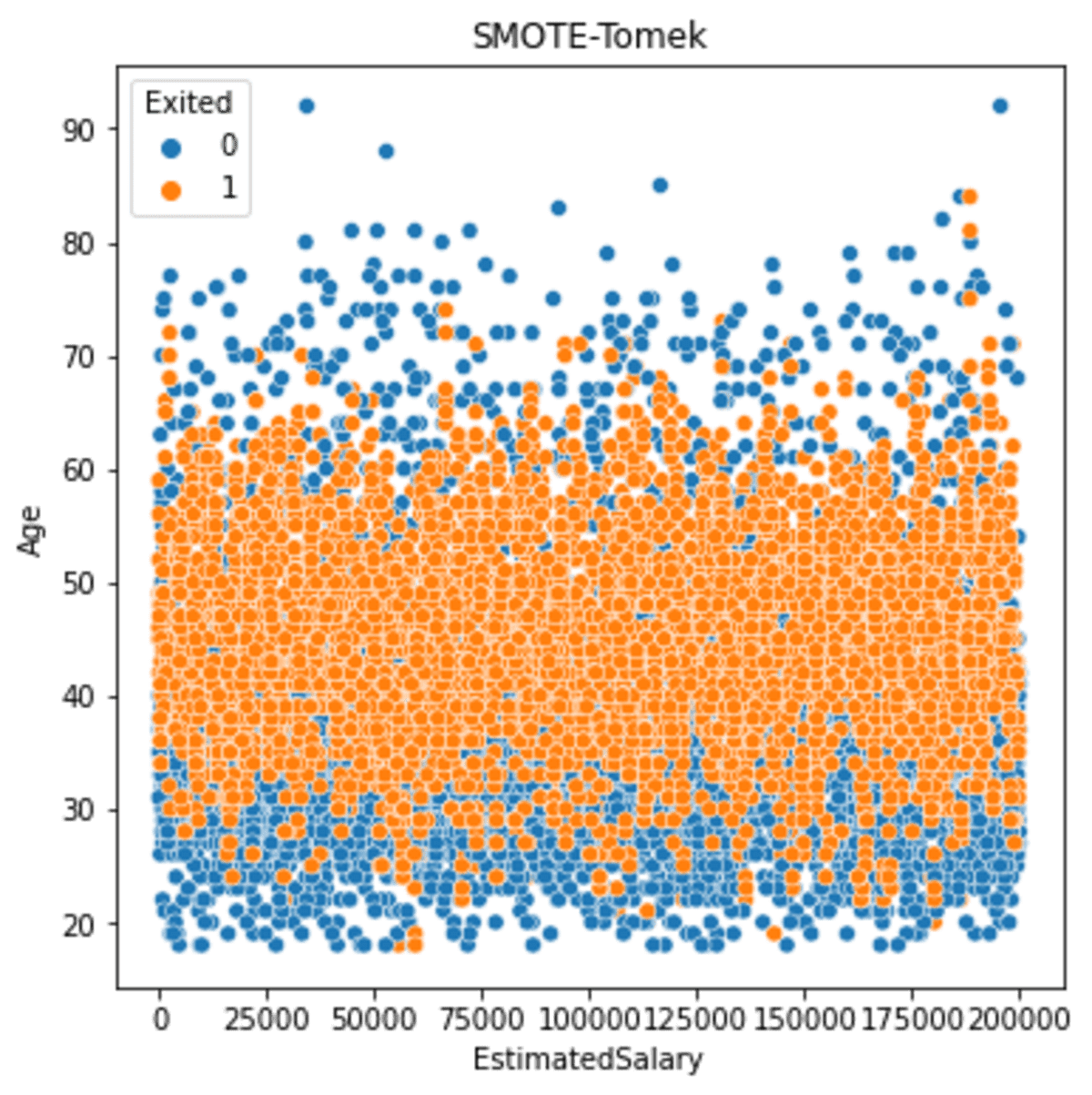
The resulting spread is still similar to before. But if we see more detail, less minority oversampled is produced the further the data is.

5. SMOTE-ENN

Similar to the SMOTE-Tomek, SMOTE-ENN (Edited Nearest Neighbour) combines oversampling and undersampling. The SMOTE did the oversampling, while the ENN did the undersampling.

The Edited Nearest Neighbour is a way to remove majority class samples in both original and sample result datasets where the nearest class minority samples5 misclassifies it. It will remove the majority class close to the border where it was misclassified.

Let’s try the SMOTE-ENN with an example dataset.

from imblearn.combine import SMOTEENN

s_enn = SMOTEENN(random_state=42)
X_se, y_se = s_enn.fit_resample(df[['EstimatedSalary', 'Age']], df['Exited'])
df_se = pd.DataFrame(X_se, columns = ['EstimatedSalary', 'Age'])
df_se['Exited'] = y_se

Let’s see the SMOTE-ENN result. First, we would take a look at the target variable.

df_se['Exited'].value_counts().plot(kind = 'bar', color = ['blue', 'red'])

The undersampling process of the SMOTE-ENN is much more strict compared to the SMOTE-Tomek. From the result above, more than half of the original 'Exited' class 0 was undersampled, and only a slight increase of the minority class.

Let’s see the data spread after the SMOTE-ENN is applied.

sns.scatterplot(data = df_se, x ='EstimatedSalary', y = 'Age', hue = 'Exited')
plt.title('SMOTE-ENN')

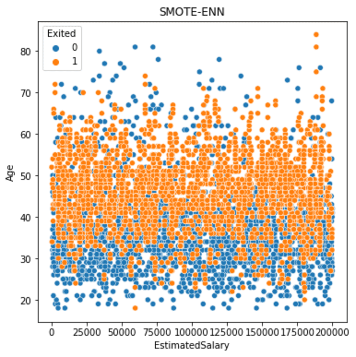
The data spread is much larger between the classes than before. However, we need to remember that the result data is smaller.

6. SMOTE-CUT

SMOTE-CUT or SMOTE-Clustered Undersampling Technique combines oversampling, clustering, and undersampling. 

SMOTE-CUT implements oversampling with SMOTE, clustering both the original and result and removing the class majority samples from clusters. 

SMOTE-CUT clustering is based on the EM or Expectation Maximization algorithm, which would assign each data with a probability of belonging to clusters. The clustering result would guide the algorithm to oversample or undersample, so the dataset distribution becomes balanced6.

Let’s try using a dataset example. For this example, we would use the crucio Python package.

pip install crucio 

With the crucio package, we oversample the dataset using the following code. 

from crucio import SCUT
df_sample = df[['EstimatedSalary', 'Age', 'Exited']].copy()

scut = SCUT()
df_scut= scut.balance(df_sample, 'Exited')

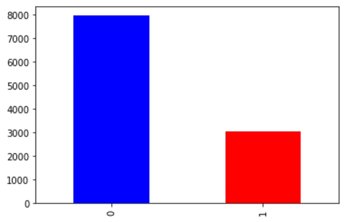
Let’s see the target data distribution.

df_scut['Exited'].value_counts().plot(kind = 'bar', color = ['blue', 'red'])

The 'Exited' class is equal, although the undersampling process is quite strict. Many of the 'Exited' class 0 were removed due to the undersampling.

Let’s see the data spread after SMOTE-CUT was implemented.

sns.scatterplot(data = df_scut, x ='EstimatedSalary', y = 'Age', hue = 'Exited')
plt.title('SMOTE-CUT')

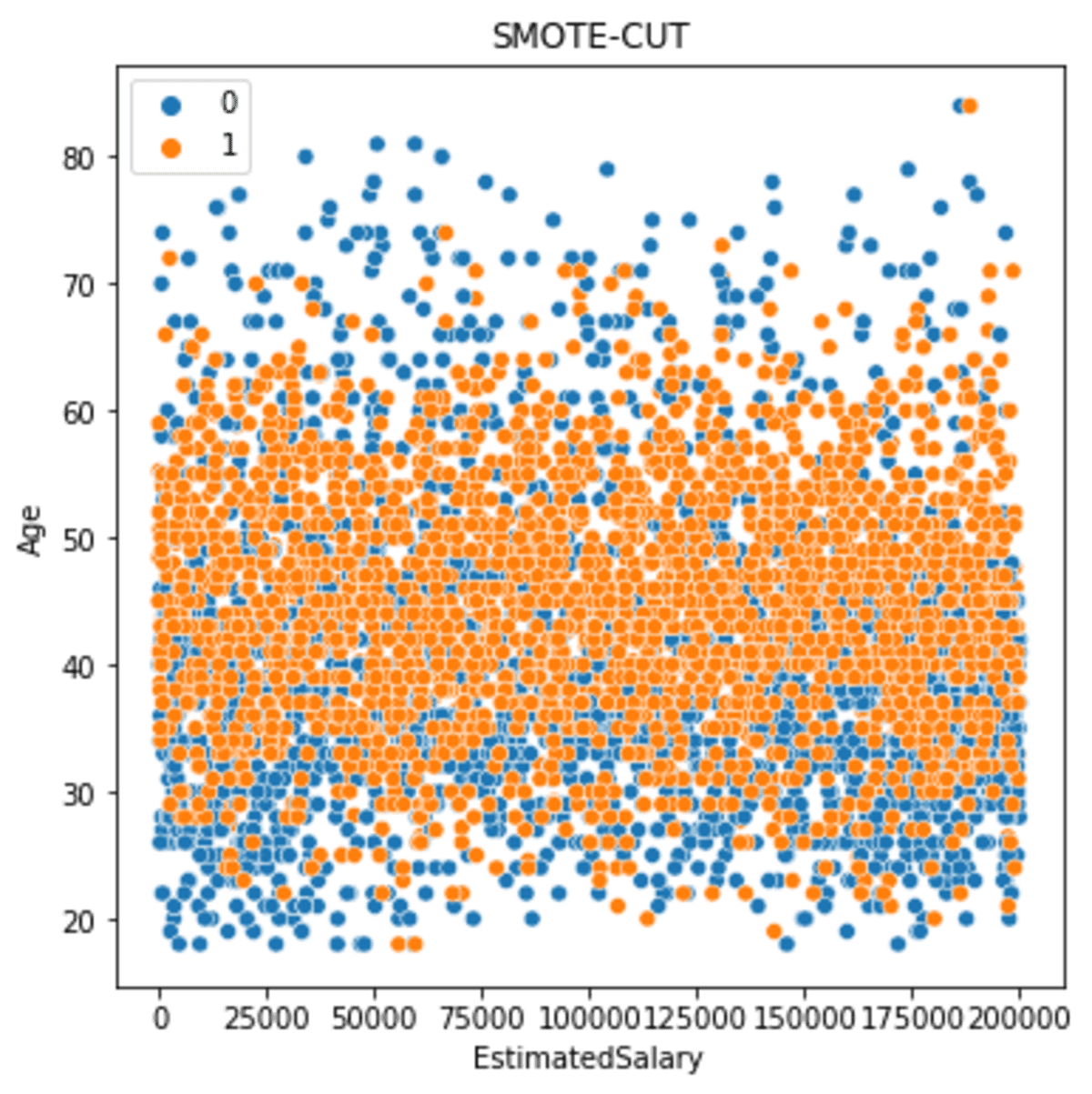
The data spread is more spread but less than the SMOTE-ENN. 

7. ADASYN

ADASYN or Adaptive Synthetic Sampling is a SMOTE that tries to oversample the minority data based on the data density. ADASYN would assign a weighted distribution to each of the minority samples and prioritize oversampling to the minority samples that are harder to learn7. 

Let’s try ADASYN with the example dataset.

from crucio import ADASYN
df_sample = df[['EstimatedSalary', 'Age', 'Exited']].copy()

ada = ADASYN()
df_ada= ada.balance(df_sample, 'Exited')

Let’s see the target distribution result.

df_ada['Exited'].value_counts().plot(kind = 'bar', color = ['blue', 'red'])

As the ADASYN would focus on the data that is harder to learn or less dense, the oversampling result was less than the other. 

Let’s see how the data spread was.

sns.scatterplot(data = df_ada, x ='EstimatedSalary', y = 'Age', hue = 'Exited')
plt.title('ADASYN')

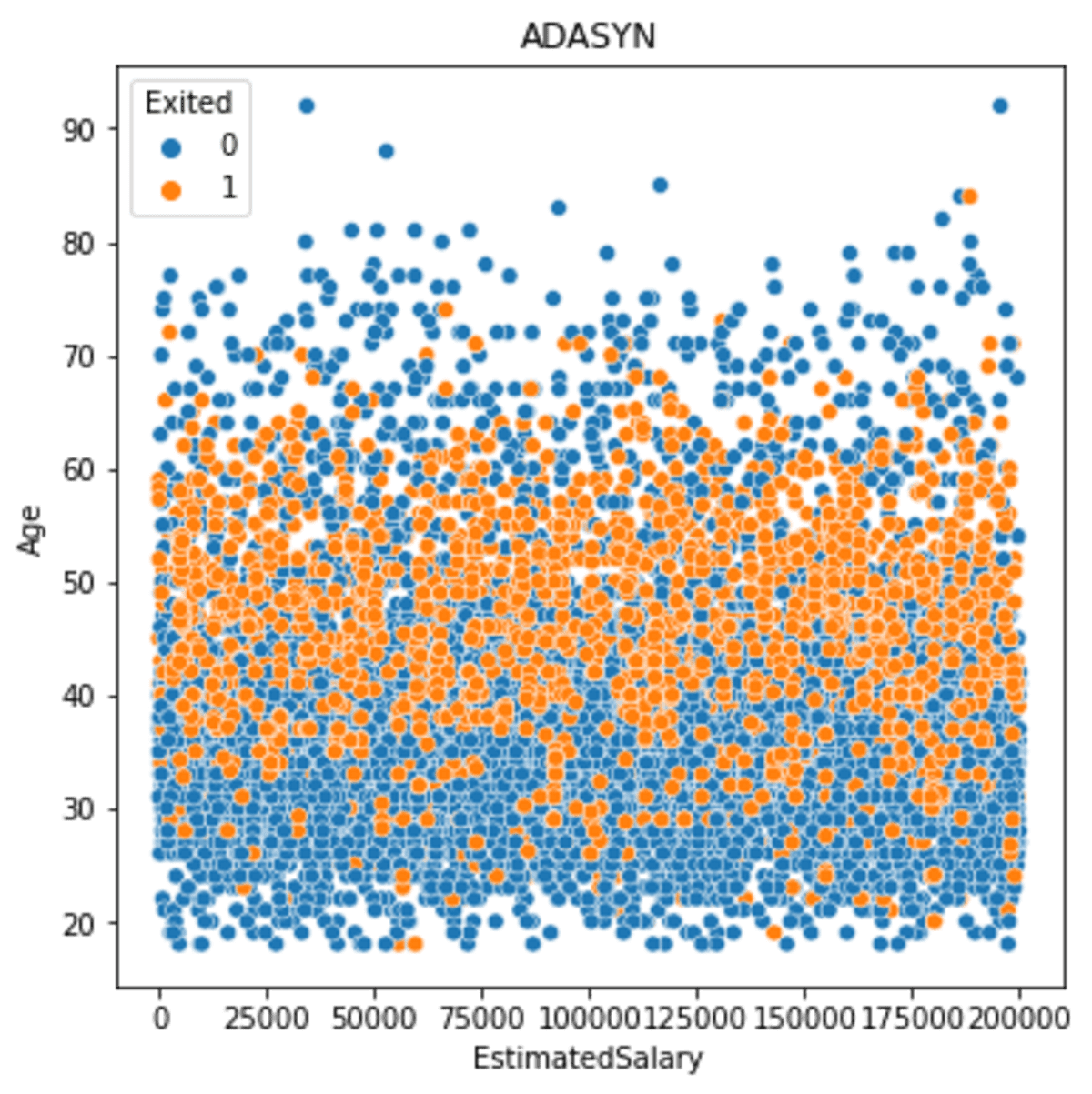
As we can see from the image above that the spread is closer to the core but closer to the low-density minority data.

Conclusion

Data imbalance is a problem in the data field. One way to mitigate the imbalance problem is by oversampling the dataset with SMOTE. With research development, many SMOTE methods have been created that we can use. 

In this article, we go through 7 different SMOTE techniques, including

1. SMOTE
2. SMOTE-NC
3. Borderline-SMOTE
4. SMOTE-TOMEK
5. SMOTE-ENN
6. SMOTE-CUT
7. ADASYN

References

1. SMOTE: Synthetic Minority Over-sampling Technique - Arxiv.org
2. Churn Modelling dataset from Kaggle licenses under CC0: Public Domain.
3. Borderline-SMOTE: A New Over-Sampling Method in Imbalanced Data Sets Learning - Semanticscholar.org
4. Balancing Training Data for Automated Annotation of Keywords: a Case Study - inf.ufrgs.br
5. Improving Risk Identification of Adverse Outcomes in Chronic Heart Failure Using SMOTE+ENN and Machine Learning - dovepress.com
6. Using Crucio SMOTE and Clustered Undersampling Technique for unbalanced datasets - sigmoid.ai
7. ADASYN: Adaptive Synthetic Sampling Approach for ImbalancedLearning - ResearchGate

 
 
Cornellius Yudha Wijaya is a data science assistant manager and data writer. While working full-time at Allianz Indonesia, he loves to share Python and Data tips via social media and writing media.