First Open Source Implementation of DeepMind’s AlphaTensor
The first open-source implementation of AlphaTensor has been released and opens the door for new developments to revolutionize the computational performance of deep learning models.

Photo by DeepMind on Unsplash
Matrix multiplication is a fundamental operation used in many systems, from neural networks to scientific computing routines. Finding efficient and provably correct algorithms for matrix multiplication can have a huge impact on making computation faster and more efficient, but is a very challenging task. The space of possible algorithms is enormous, and traditional methods for discovering algorithms, such as human-designed heuristics or combinatorial search, are often suboptimal.
DeepMind's recently proposed AI-based solution for automated search goes far beyond human intuition. The solution consists of a deep reinforcement learning agent called AlphaTensor, built on top of AlphaZero. This agent is trained to play a single-player game, TensorGame, where the goal is to discover computationally efficient algorithms for matrix multiplication.
AlphaTensor is particularly good at handling large matrices by decomposing large matrix multiplications into smaller multiplications. Moreover, AlphaTensor can be used to achieve state-of-the-art performance for matrix multiplication once fine-tuned on a specific hardware device.
AlphaTensor has great potential for accelerating deep learning computing. In deep learning, many time-consuming operations can be mapped to matrix multiplications. By using AlphaTensor to optimize these operations, the overall performance of deep learning models can be significantly improved.
Recently, OpenAlphaTensor, the first open source implementation of AlphaTensor, was released, which could revolutionize the computational power of deep learning models.
Matrix Multiplication Tensor
For non-experts in matrix multiplication optimization, it may not be straightforward to understand how an operation such as matrix multiplication can be mapped in a three-dimensional tensor. I will try to explain it in simple words and with examples.
Let’s consider the product C = A*B, where for simplicity both A and B are square matrices of size N. The multiplication operation can be mapped in a 3D tensor of shape (N^2, N^2, N^2). The first tensor dimension represents the flattened matrix A, the second dimension the flattened matrix B and the third dimension the flattened matrix C.
The tensor has only binary values (either 1 or 0) for each entry. Note that the tensor represents the multiplication operation, so it is independent of the values of the matrices A and B.
Every entry of the tensor corresponds to the coefficient of the operation. For example, to compute C[1,1], it is necessary to multiply both A[1,1] and B[1,1]. Therefore, the tensor entry [0,0,0], which corresponds to A[1,1], B[1,1] and C[1,1], will have value 1. In contrast, to compute C[1,1], A[2,1] is not needed. Thus, the tensor row T[N+1, :, 0] will contain only zeros.
The image below shows an example of a tensor for N=2.
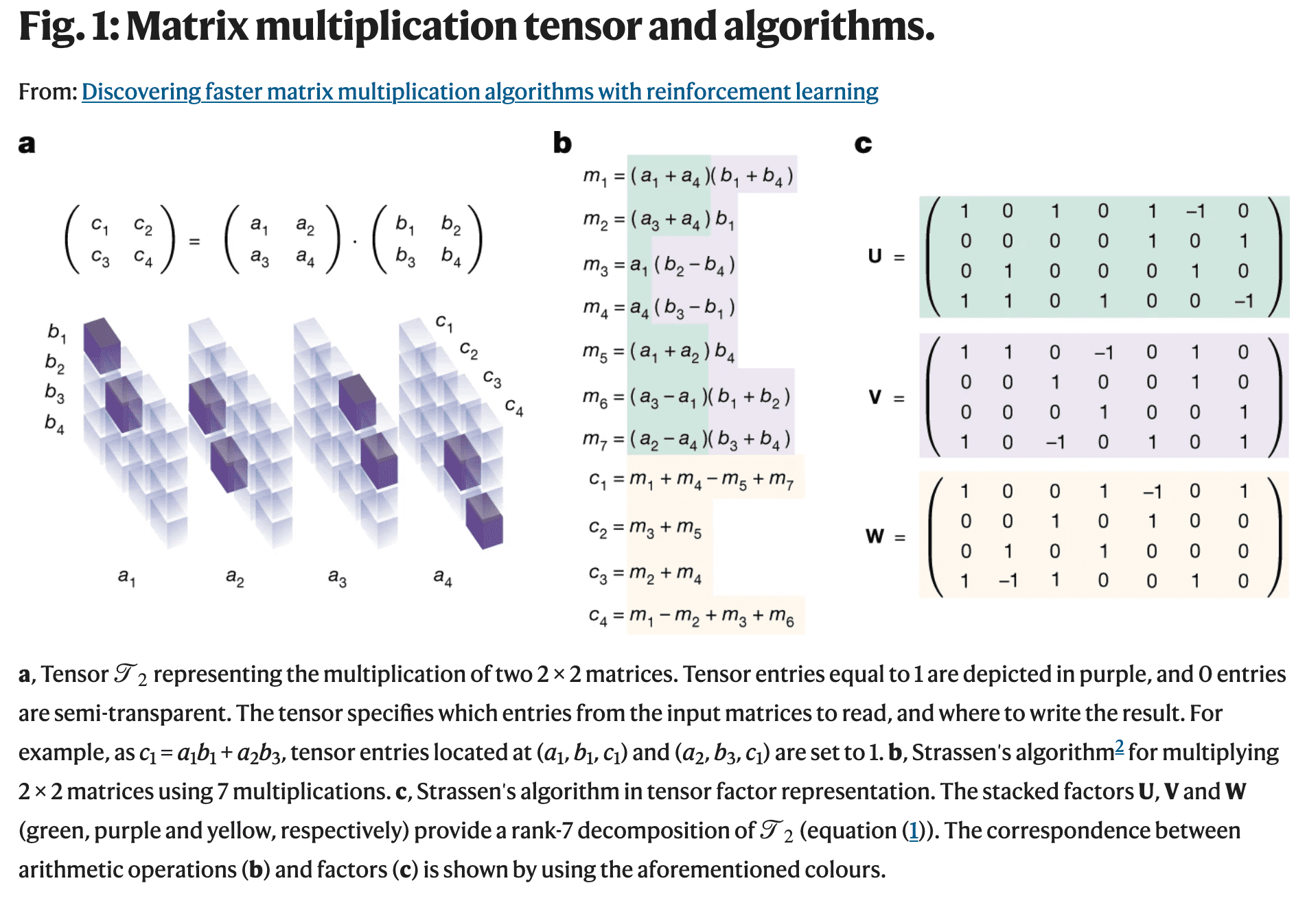
Image from DeepMind's paper published in Nature
As shown in (b) and (c) in the figure above, it is possible to implement an algorithm for computing the product using a decomposition of the 3D tensor. More specifically, the algorithm below can be used for converting a tensor decomposition (the matrices U, V, W) into a matrix multiplication algorithm.

Meta-algorithm parameterized for computing the matrix product C=AB introduced in DeepMind's paper
The TensorGame
The problem of finding efficient algorithms for matrix multiplication is extremely challenging because the number of possible algorithms to consider is much larger than the number of atoms in the universe, even for small instances of matrix multiplication.
DeepMind converted this problem into a single-player game, and called it the TensorGame. In this game, the player chooses how to combine different entries of matrices to multiply them. A score is assigned based on the number of operations required to achieve the correct multiplication result. The game ends when the zero tensor is reached or when the maximum number of moves has been made. The final factorization is evaluated based on an estimation of the residual rank and certain optimization criteria, such as asymptotic time complexity or practical runtime.
The initial position in the TensorGame corresponds to the Matrix Multiplication Tensor expressed on some random basis.
In each step t of the game, the player writes down three vectors  , which specifies the rank-1 tensors . The state of the game is updated by subtracting the vectors selected by the player:

where is the Matrix Multiplication Tensor.
If the game ends in p steps, this means that the Matrix Multiplication Tensor can be decomposed into p rank-1 tensors , i.e. it has at least rank p.
The TensorGame can then be interpreted as a rank-decomposition algorithm and AlphaTensor can be seen as an algorithm for estimating the rank of the tensor.
AlphaTensor Architecture
So far we have learned about the TensorGame and clarified how its solution can be seen as a matrix multiplication algorithm. Let’s now explore the main concepts of AlphaTensor, the algorithm used for the game.
AlphaTensor architecture is basically an encoder-decoder Transformer architecture where:
- the encoder takes as input the game state , the n previous actions taken by the model (usually n=7), and the time index t of the current action. Information is stacked together in a tensor with shape (n+1, N^2, N^2, N^2). This tensor is then reshaped and transformed (using three linear layers) in a tensor of shape (N^2, N^2, c) where c is the inner dimension of the model.
- the decoder generates the n_steps actions from the embedded vector given by the encoder in an auto-regressive way. Each action corresponds to a token of the triplets representing one of the triplets decomposing the game tensor (i.e. reducing its rank)
The model is trained by alternating back-propagation and model acting. Model acting is used to generate data that is then used to train the model. In practice, the model is trained with a mixture of synthetically generated data and data generated by the model during acting. The acting step is done by taking a 3D tensor corresponding to a matrix operation and playing n_actors games on it. Each actor plays a game either on the standard basis or on an alternative basis (the change of basis is applied with a given probability). The results are then collected and can be used in the training step with the synthetic data.
The acting step is based on AlphaZero's Monte Carlo Tree Search (MCTS), modified to support large action spaces. In short, before choosing the action, n_sims paths are explored from the model output with a maximum future exploration of 5 steps. The probabilities generated by the model are then adjusted taking into account the generated paths. Then the action with the most promising future path(s) is chosen to continue the game.
While training the model, the reward is actually a negative reward (penalty). Its absolute value increases with each additional step required to solve the game. If the model takes m steps to solve a TensorGame, the reward associated with the game is r=-m. If the model is not able to solve the TensorGame in max_rank steps, the reward is computed by estimating the rank of the remaining tensor. The rank is estimated as the sum of the ranks of the matrices that compose the tensor. The estimate is an upper bound on the true rank of the tensor.
When fine-tuning the model, the penalty reward at the terminal state should also take into account the latency of the algorithm produced by the model. The reward formula becomes rt'=rt+λbt, where rt is the reward scheme described earlier, bt is the benchmark reward (non-zero only at the terminal state), and λ is a user-specified coefficient.

Speed-ups (%) of AlphaTensor-discovered algorithms tailored for a GPU and a TPU, extracted from DeepMind’s paper. Speed-ups are measured relative to standard (e.g. cuBLAS for the GPU) matrix multiplication on the same hardware and compared to the Strassen-square algorithm. Source: DeepMind.
The Open Source Implementation of DeepMind’s AlphaTensor
I recently released OpenAlphaTensor, the first open source implementation of AlphaTensor. In this section I will walk through the implementation. As we discussed earlier, the AlphaTensor architecture is fairly straightforward, based on a standard transformer with an encoder-decoder architecture. The most interesting components of AlphaTensor are the first layer in the encoder part and the way the actions are sampled.
Let’s start with the first encoding layer.
# x.size = (N, T, S, S, S)
# scalars.size = (N, s)
batch_size = x.shape[0]
S = x.shape[-1]
T = x.shape[1]
x1 = x.permute(0, 2, 3, 4, 1).reshape(batch_size, S, S, S * T)
x2 = x.permute(0, 4, 2, 3, 1).reshape(batch_size, S, S, S * T)
x3 = x.permute(0, 3, 4, 2, 1).reshape(batch_size, S, S, S * T)
input_list = [x1, x2, x3]
for i in range(3):
    temp = self.linears_1[i](scalars).reshape(batch_size, S, S, 1)
    input_list[i] = torch.cat([input_list[i], temp], dim=-1)
    input_list[i] = self.linears_2[i](input_list[i])
x1, x2, x3 = input_list
In the snippet above, we show how the input tensor is decomposed into three tensors, which are then used as query, key, and value inputs of the transformer-layer.
- Across the three tensor dimensions representing the flattened matrices (A, B, C), the input tensor is flattened along each dimension together with the dimension representing the previous actions. In this way, in each flattened-copy of the input tensor, the selected dimension is an aggregation of the last T-1 values and the actual value, for all the S values of the selected dimension, where S=N^2. Philosophically, it is as if, for each dimension, we focus on what happened in the previous actions in that dimension.
- The scalars are mapped in three different spaces of dimension S^2, and then reshaped to be concatenated with the tensors obtained at the previous point. Conceptually, the scalars are mapped to an embedding space of dimension S^2, and then the embedded information is chunked into S vectors and stacked together, similar to what happens to text when tokenized.
- Scalar tokens are concatenated with the restructured input tensor and then given as input to a linear layer for mapping the scalars+channel-history focus information in the internal dimension of the model.
These three steps can be interpreted as a way of giving to the model both information about the scalars (as in the TensorGame time step) and the focus on the previous actions for each channel.
Regarding the way the actions are produced, it is interesting to note that AlphaTensor generates as output the triplet u, v, w, which aims to reduce the tensor rank. The three vectors have size S and since they are concatenated the model has to produce a vector of size 3*S. AlphaTensor is trained with a RL algorithm, so all possible actions must be expressed in terms of probabilities in an enumerated space, i.e. the model produces a probability over the different actions. This means that each vector in the 3S space should be mapped to a different action. This results in an action space of size |F|^(3S), where |F| is the number of different values that the element of u, v, w can take. Usually, the values are restricted to (-2, -1, 0, 1, 2), resulting in a cardinality of 5 elements.
Here comes a major challenge: to generate the action probabilities for a matrix product of matrices of size 5 we would need a memory of 5^75 * 4 bytes, which would mean ~10^44 GB of memory. Clearly, we cannot manage such a large action space.
How do we solve the problem? To reduce the memory footprint of the action probabilities we can split the triplets into smaller chunks, “tokenize” them, and treat the chunks as generated tokens in the transformer architecture, i.e. the tokens are given as input to the decoder in an auto-regressive way. In the example above we can split the triplets into 15 chunks, reducing the memory consumption to 15 * 5^(75/15) * 4, i.e. 187.5 KB.
def _eval_forward(self, e: torch.Tensor):
    bs = e.shape[0]
    future_g = (
        torch.zeros((bs, self.n_samples, self.n_steps)).long().to(e.device)
    )
    ps = torch.ones((bs, self.n_samples)).to(e.device)
    e = e.unsqueeze(1).repeat(1, self.n_samples, 1, 1)

    future_g = future_g.view(-1, self.n_steps)
    ps = ps.view(-1)
    e = e.view(-1, e.shape[-2], e.shape[-1])
    for i in range(self.n_steps):
        o_s, z_s = self.core(future_g[:, : i + 1], e)
        future_g[:, i], p_i = sample_from_logits(o_s[:, i])
        ps *= p_i
    future_g = future_g.view(bs, self.n_samples, self.n_steps)
    ps = ps.view(bs, self.n_samples)
    return (
        future_g,
        ps,
        z_s[:, 0].view(bs, self.n_samples, *z_s.shape[2:]).mean(1),
    )
Above we show the code snippet for generating the full action. In the code, self.core contains the decoder layer and the tensor e represents the output of the encoder layer. Zero can be considered as the <eos> token in NLP models and the n_steps actions representing the n_steps chunks are generated in a progressive way.
The model returns three quantities:
- The generated actions
- The probability associated to the full action
- The logits produced for generating the first action (the first chunk) that will be used for computing the model value.
It is worth spending a few words on the n_samples parameter. The parameter is used for the acting step and it allows the model to generate different versions of the triplets which will then be used for exploring the action space in the Monte Carlo Tree Search algorithm used in the Acting process. The n_samples different actions are sampled according to the policy generated by the model.
Acting Step
The most tricky part of the whole algorithm is probably the Acting step used for solving the TensorGame. The algorithm is not deeply explained in the AlphaTensor paper, since it is based on several DeepMind’s previous papers which are just cited and given as known. Here, I’ll reconstruct all the missing pieces and explain step by step our implementation.
We can organize the acting steps in three different components:
- The Monte-Carlo Tree Search
- The game simulation
- The Improved policy computation
Let us analyze them one by one.
Monte-Carlo Tree Search (MCTS)
Monte Carlo Tree Search (MCTS) is a widely used artificial intelligence technique for game playing, particularly in board games and video games. The algorithm creates a game tree that simulates potential moves and outcomes and uses random sampling to evaluate the expected reward for each move. The algorithm then iteratively selects the move with the highest expected reward and simulates outcomes until it reaches a terminal state or a specified stopping condition. The simulations are used to estimate the probability of winning for each move and guide the decision-making process. MCTS has been shown to be effective in complex games where the number of possible moves and outcomes is large, and it has been used in successful game-playing AI systems, such as AlphaGo.
In AlphaTensor a modified version of the original MCTS is used. In particular, instead of randomly selecting the action from the whole action space, the action is selected among a subset generated directly by the model (through the n_samples presented before). The correction to the policy upgrade is then applied in the Improved Policy computation step.
In our implementation, we decided to keep all the information about the Monte-Carlo tree in a dictionary having as key the hash-version of the TensorGame state and as values the information associated with the state itself. Each Monte-Carlo step starts from a node and simulates n_sim mini-games, exploring the future with a horizon of 5 moves. If the node has already been explored in previous simulations, n_sim is adjusted considering the number of previous explorations. For each node the number of visits is stored in the N_s_a tensor, since this tensor contains the number of visits per node child action (among the ones sampled by the model).
def monte_carlo_tree_search(
    model: torch.nn.Module,
    state: torch.Tensor,
    n_sim: int,
    t_time: int,
    n_steps: int,
    game_tree: Dict,
    state_dict: Dict,
):
"""Runs the monte carlo tree search algorithm.

    Args:
        model (torch.nn.Module): The model to use for the simulation.
        state (torch.Tensor): The initial state.
        n_sim (int): The number of simulations to run.
        t_time (int): The current time step.
        n_steps (int): The maximum number of steps to simulate.
        game_tree (Dict): The game tree.
        state_dict (Dict): The dictionary containing the states.
    """
    state_hash = to_hash(extract_present_state(state))
    if state_hash in state_dict:
        with torch.no_grad():
            N_s_a = state_dict[state_hash][3]
            n_sim -= int(N_s_a.sum())
            n_sim = max(n_sim, 0)

    for _ in range(n_sim):
        simulate_game(model, state, t_time, n_steps, game_tree, state_dict)
    # return next state
    possible_states_dict, _, repetitions, N_s_a, q_values, _ = state_dict[
        state_hash
    ]
    possible_states = _recompose_possible_states(possible_states_dict)
    next_state_idx = select_future_state(
        possible_states, q_values, N_s_a, repetitions, return_idx=True
    )
    next_state = possible_states[next_state_idx]
    return next_state
The code above shows our implementation of the algorithm. For a matter of code simplicity, the policy correction is performed in the simulate_game function.
Game Simulation
The simulate_game function is responsible for exploring the tree composed of nodes representing a particular state of the TensorGame. It also runs the model whenever a leaf node is encountered and it stores all node information in the state_dict dictionary. Let’s give a deep look at its implementation:
@torch.no_grad()
def simulate_game(
    model,
    state: torch.Tensor,
    t_time: int,
    max_steps: int,
    game_tree: Dict,
    states_dict: Dict,
    horizon: int = 5,
):
"""Simulates a game from a given state.

  Args:
      model: The model to use for the simulation.
      state (torch.Tensor): The initial state.
      t_time (int): The current time step.
      max_steps (int): The maximum number of steps to simulate.
      game_tree (Dict): The game tree.
      states_dict (Dict): The states dictionary.
      horizon (int): The horizon to use for the simulation.
  """
  idx = t_time
  max_steps = min(max_steps, t_time + horizon)
  state_hash = to_hash(extract_present_state(state))
  trajectory = []
  # selection
  while state_hash in game_tree:
      (
          possible_states_dict,
          old_idx_to_new_idx,
          repetition_map,
          N_s_a,
          q_values,
          actions,
      ) = states_dict[state_hash]
      possible_states = _recompose_possible_states(possible_states_dict)
      state_idx = select_future_state(
          possible_states, q_values, N_s_a, repetition_map, return_idx=True
      )
      trajectory.append((state_hash, state_idx))  # state_hash, action_idx
      future_state = extract_present_state(possible_states[state_idx])
      state = possible_states[state_idx]
      state_hash = to_hash(future_state)
      idx += 1

  # expansion
  if idx <= max_steps:
      trajectory.append((state_hash, None))
      if not game_is_finished(extract_present_state(state)):
          state = state.to(model.device)
          scalars = get_scalars(state, idx).to(state.device)
          actions, probs, q_values = model(state, scalars)
          (
              possible_states,
              cloned_idx_to_idx,
              repetitions,
              not_dupl_indexes,
          ) = extract_children_states_from_actions(
              state,
              actions,
          )
          not_dupl_actions = actions[:, not_dupl_indexes].to("cpu")
          not_dupl_q_values = torch.zeros(not_dupl_actions.shape[:-1]).to(
              "cpu"
          )
          N_s_a = torch.zeros_like(not_dupl_q_values).to("cpu")
          present_state = extract_present_state(state)
          states_dict[to_hash(present_state)] = (
              _reduce_memory_consumption_before_storing(possible_states),
              cloned_idx_to_idx,
              repetitions,
              N_s_a,
              not_dupl_q_values,
              not_dupl_actions,
          )
          game_tree[to_hash(present_state)] = [
              to_hash(extract_present_state(fut_state))
              for fut_state in possible_states
          ]
          leaf_q_value = q_values
  else:
      leaf_q_value = -int(torch.linalg.matrix_rank(state).sum())
  # backup
  backward_pass(trajectory, states_dict, leaf_q_value=leaf_q_value)
Each simulation is divided in three parts:
- Selection
- Expansion
- Backup
In the selection part the simulation is run on the already generated tree-nodes, and the following node is selected using the following function:
def select_future_state(
    possible_states: List[torch.Tensor],
    q_values: torch.Tensor,
    N_s_a: torch.Tensor,
    repetitions: Dict[int, list],
    c_1: float = 1.25,
    c_2: float = 19652,
    return_idx: bool = False,
) -> torch.Tensor:
"""Select the future state maximizing the upper confidence bound."""
# q_values (1, K, 1)
    pi = torch.tensor(
        [
            len(repetitions[i])
            for i in range(len(possible_states))
            if i in repetitions
        ]
    ).to(q_values.device)
    ucb = q_values.reshape(-1) + pi * torch.sqrt(
        torch.sum(N_s_a) / (1 + N_s_a)
    ) * (c_1 + torch.log((torch.sum(N_s_a) + c_2 + 1) / c_2))
    if return_idx:
        return ucb.argmax()
    return possible_states[ucb.argmax()]
In practice, the action maximizing the ucb function:
for the given state is selected. Here Q represents the Q values generated by the model and π represents the random distribution over the actions sampled using the model policy. N(s, a) represents the number of visits of the node to action a from node s.
Once the selection phase reaches a leaf node, if the simulation has not reached a terminal condition (in terms of either maximum exploration, i.e. future horizon, or game ending), the model is then used for selecting n_samples alternative nodes (they will be leaf nodes in the successive iteration). This is called the expansion phase, since new nodes are added to the tree. Then, no further node is explored in the current simulation, but the leaf q_value is sent to the following simulation step: the backup.
Backup is the final stage of each simulation. During backup, if the leaf node was a terminal state the final reward is computed; otherwise the leaf q value is used as an estimated reward. Then the reward is back-propagated on the simulation trajectory updating both the states q_values and updating the visit counter N(s, a). In the snippet below we show the code for the reward back-propagation.
def backward_pass(trajectory, states_dict, leaf_q_value: torch.Tensor):
"""Backward pass of the montecarlo algorithm"""
reward = 0
    for idx, (state, action_idx) in enumerate(reversed(trajectory)):
        if action_idx is None:  # leaf node
            reward += leaf_q_value
        else:
            (
                _,
                old_idx_to_new_idx,
                _,
                N_s_a,
                q_values,
                _,
            ) = states_dict[state]
            if isinstance(reward, torch.Tensor):
                reward = reward.to(q_values.device)
            action_idx = int(action_idx)
            if action_idx in old_idx_to_new_idx:
                not_dupl_index = old_idx_to_new_idx[int(action_idx)]
            else:
                not_dupl_index = action_idx
            reward -= 1
            q_values[:, not_dupl_index] = (
                N_s_a[:, not_dupl_index] * q_values[:, not_dupl_index] + reward
            ) / (N_s_a[:, not_dupl_index] + 1)
            N_s_a[:, not_dupl_index] += 1
Improved Policy Computation
Once all the simulations have been run and the MCTS offers an interesting snapshot of the near future it is time to update the policy associated with the predicted nodes and return them, so that they can be used during training. The improved policy, following the method described in Hubert et al, is used for managing large action spaces. In fact, for small search space, it is possible during MCTS to sample an action randomly from the action space and evaluate its impact. A similar approach in a much larger action space would lead to all trajectories diverging in different paths and it would need an infinite amount of trajectories for getting meaningful statistics and then updating the policy. Since here we are using sample-MCTS for avoiding the dispersion, i.e. n_samples actions are sampled accordingly to the model policy and then MCTS just selects one of the sampled actions while exploring the tree, we need to take into account the sample-correction when computing the final updated policy that will be used while training the model.
In practice, the improved policy is computed as

where
def compute_improved_policy(
state_dict: Dict,
states: List[str],
model_n_steps: int,
model_n_logits: int,
N_bar: int,
):
"""Compute the improved policy given the state_dict, the list of states.
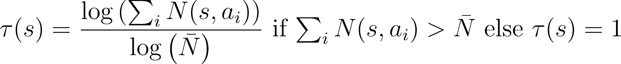
The improved policy is computed as (N_s_a / N_s_a.sum())^(1/tau) where tau
is (log(N_s_a.sum()) / log(N_bar)) if N_s_a.sum() > N_bar else 1.
"""
policies = torch.zeros(len(states), model_n_steps, model_n_logits)
N_bar = torch.tensor(N_bar)
for idx, state in enumerate(states):
N_s_a = state_dict[state][3]
actions = state_dict[state][5]
if N_s_a.sum() > N_bar:
tau = (torch.log(N_s_a.sum()) / torch.log(N_bar)).item()
else:
tau = 1
N_s_a = N_s_a ** (1 / tau)
improved_policy = N_s_a / N_s_a.sum()
for sample_id in range(actions.shape[1]):
action_ids = actions[0, sample_id]
for step_id, action_id in enumerate(action_ids):
policies[idx, step_id, action_id] += improved_policy[
0, sample_id
]
return policies
Note that in our implementation after having computed the policy from the N_s_a tensor we have to map it back to the original action tensor. In fact, N_s_a just considers the actions sampled by the model, while the final policy must contain probabilities also for the not-explored actions.
Differences with respect to ChatGPT training algorithm
AlphaTensor is the latest member of the AlphaGo/AlphaZero family of artificial intelligence methods by DeepMind. These methods are based on the Monte Carlo Tree Search (MCTS) algorithm, which has been refined and enhanced by DeepMind to tackle increasingly complex tasks. Another AI system, OpenAI's ChatGPT, which has caused a lot of buzz for its remarkable performance, was trained with a different approach, called Reinforcement Learning with Human Feedback (RLHF).
RLHF is a fine-tuning technique used to tune language models to follow a set of written instructions. It uses human preferences as a reward signal to fine-tune the model, thereby aligning the behavior of the language model with the stated preferences of a specific group of people, rather than some broader notion of ‘human values’.
In contrast, MCTS is a tree-based search algorithm used to determine the optimal moves in games. It simulates potential moves and updates the values of each move based on their outcomes, guiding the selection of the best move.
RLHF collects data from human-written demonstrations and human-labeled comparisons between AI models, and trains a reward model to predict the preferences of a given group of people. The reward model is then used to fine-tune the AI models. MCTS, on the other hand, uses simulations and evaluations to determine the best decision.
Although they are different approaches, RLHF and MCTS also have similarities. Both artificial intelligence techniques use decision-making and problem solving methods, and both use a trial-and-error approach to explore different options and make decisions based on available information. Both are also iterative processes that improve over time as more information and experience are gathered.
The choice between RLHF and MCTS depends on the task at hand. RLHF is ideal when there is no clear metric for evaluating the model performance, while MCTS has proven effective in game-like tasks where knowledge and exploration of the future give the model a significant advantage.
Code Optimization for AlphaTensor training
Implementing the AlphaTensor training algorithm requires finding the perfect compromise between training speed and memory consumption. As seen in the Model section, simply considering the action tokenization can save a lot of memory, but an overly aggressive action space reduction can lead to both drop in accuracy and slower performance. The latter happens because all tokens are generated sequentially in an autoregressive way by the model decoder. Therefore, the inference time grows linearly with the number of tokens per action once the softmax on the action space is not the bottleneck anymore.
When setting up AlphaTensor training, the main difficulties were found in dealing with the acting process. If the tensors are not stored in the correct format, the MCTS can easily cause uncontrolled memory usage growth. On the other hand, if the number of tensors stored during each simulation is reduced too much, the MCTS can spend an infinite amount of time re-computing the required states.
Let's take an example of the game simulation step, where the game is explored by looking at possible future scenarios. For each state, if we don't save the actions generated by the model and we decide to save only the random seed used to sample the actions from the policy, then each time we explore a tree node we would have to recompute the policy and then sample the actions. Clearly, we decided to store the sampled actions to save time and to avoid having to manage model sharing between different processes in the case of MCTS exploration parallelization. However, just saving the actions was not enough to get a sufficiently efficient acting step. In fact, the time for converting the n_steps actions into the (u, v, w) triplet, reducing the game tensor state and creating the new3D tensors from the n_samples actions would easily be a bottleneck for the whole training. Secondly, we didn't want to store all possible future states for each sampled action, as this would have a huge impact on the memory used by the algorithm. Suppose we set n_samples=32, n=7 and N=5, and let's remember that N is the size of the square matrix product we want to reduce and n is the number of previous actions remembered by the model. In this situation, each state tensor would have the form (8, 25, 25, 25), which multiplied by 32 would result in 3282525254 bytes for each node in the graph. Now, considering that each simulation in the expansion phase generates a new node (and n_sim=200), we would have a final memory consumption of 200328252525*4 = 3.2GB for the first MCTS node alone. In the worst-case scenario, while exploring acting max_rank nodes (where max_rank=150), this would result in a total memory consumption of 150 * 3.2GB = 480GB in RAM memory (or GPU memory if all tensors were stored on the GPU). We ran the training on our workstation with 128 GB of RAM and 48 GB of GPU memory, so we had to reduce the memory consumption.
Since we didn't want to increase the execution time, we adopted an optimization that exploits the redundancy in the state tensors produced. In fact, the tensors have n-1 previous actions in common, which can then be stored once and not repeated for each stored tensor. This results in a memory reduction of 2/7~28%, meaning that in the worst-case 137GB can be stored. At this point, by simply pruning the unused part of the tree (such as the unselected trajectories) and storing the tensors in CPU memory, we were able to avoid any memory error during training.
Next Steps
With OpenAlphaTensor now being open source, several exciting avenues for further development open up.
A natural progression is the fine-tuning of OpenAlphaTensor on target hardware devices. This is expected to lead to very competitive computational performance. I will publish more about the performance of OpenAlphaTensor on various hardware on GitHub. At the time of writing this article, OpenAlphaTensor was undergoing training.
Another important advance would be the support for remote compilation, allowing users to build algorithms optimized for edge devices. This can be achieved by storing the OpenAlphaTensor model on a server, while the matrix multiplication algorithm is evaluated on different hardware.
It could also be important to extend support for different compilers to compute the latency-based reward correction. Different compilers can lead to different optimized algorithms on a given hardware. For example, the DeepMind paper showed promising results using JAX and the XLA compiler on TPU and Nvidia GPUs. It would be interesting to evaluate this using NCCL on Nvidia or LLVM on CPUs.
Finally, extending the model and training algorithm to support larger matrix sizes remains a major open challenge. Currently, OpenAlphaTensor supports a maximum matrix size of 5, but it can be applied by splitting larger matrix multiplications into groups of tiny MMs with a size smaller than 5. This approach is suboptimal, and performing the reduction directly on the large tensor corresponding to the full MM could theoretically lead to better results.
Diego Fiori is the CTO of Nebuly AI, a company committed to making AI optimization part of every developer's toolkit.