Jupyter Notebook Best Practices for Data Science
Check out this overview of Jupyter notebook best practices as pertains to data science. Novice or expert, you may find something of use here.
By Jonathan Whitmore, Silicon Valley Data Science.
The Jupyter Notebook is a fantastic tool that can be used in many different ways. Because of its flexibility, working with the Notebook on data science problems in a team setting can be challenging. We present here some best-practices that SVDS has implemented after working with the Notebook in teams and with our clients—and that might help your data science teams as well.
![]()
The need to keep work under version control, and to maintain shared space without getting in each other’s way, has been a tricky one to meet. We present here our current view into a system that works for us—and that might help your data science teams as well.
Overall thought process
There are two kinds of notebooks to store in a data science project: the lab notebook and the deliverable notebook. First, there is the organizational approach to each notebook.
Lab (or dev) notebooks:
Let a traditional paper laboratory notebook be your guide here:
- Each notebook keeps a historical (and dated) record of the analysis as it’s being explored.
- The notebook is not meant to be anything other than a place for experimentation and development.
- Each notebook is controlled by a single author: a data scientist on the team (marked with initials).
- Notebooks can be split when they get too long (think turn the page).
- Notebooks can be split by topic, if it makes sense.
Deliverable (or report) notebooks
- They are the fully polished versions of the lab notebooks.
- They store the final outputs of analysis.
- Notebooks are controlled by the whole data science team, rather than by any one individual.
Version control
Here’s an example of how we use git and GitHub. One beautiful new feature of Github is that they now render Jupyter Notebooks automatically in repositories.
When we do our analysis, we do internal reviews of our code and our data science output. We do this with a traditional pull-request approach. When issuing pull-requests, however, looking at the differences between updated .ipynb files, the updates are not rendered in a helpful way. One solution people tend to recommend is to commit the conversion to .py instead. This is great for seeing the differences in the input code (while jettisoning the output), and is useful for seeing the changes. However, when reviewing data science work, it is also incredibly important to see the output itself.
For example, a fellow data scientist might provide feedback on the following initial plot, and hope to see an improvement:
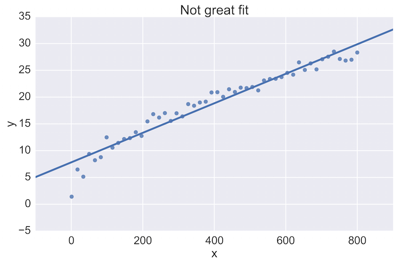
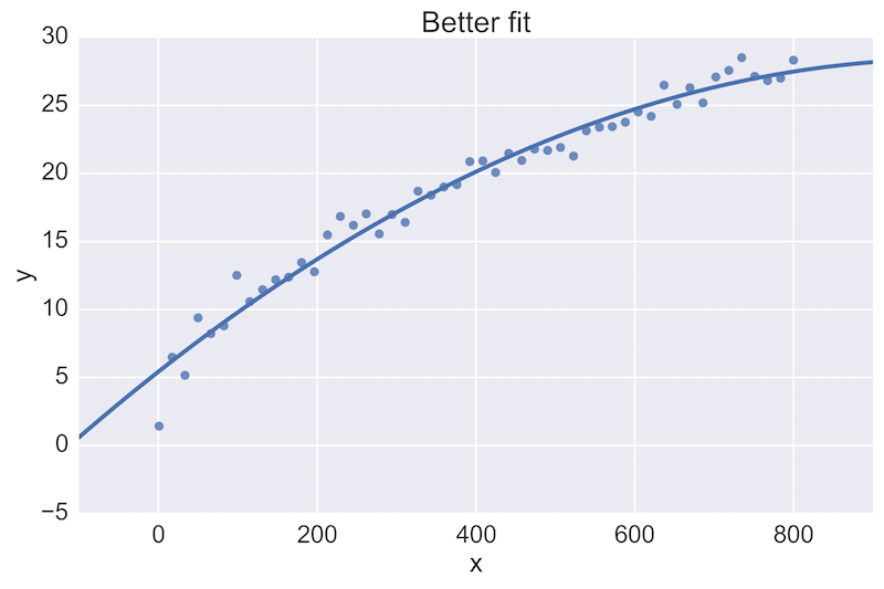
The plot on the top is a rather poor fit to the data, while the plot on the bottom is better. Being able to see these plots directly in a pull-request review of a team-member’s work is vital.
See the Github commit example here.
Note that there are three ways to see the updated figure (options are along the bottom).
Post-save hooks
We work with many different clients. Some of their version control environments lack the nice rendering capabilities. There are options for deploying an instance of nbviewer behind the corporate firewall, but sometimes that still is not an option. If you find yourself in this situation, and you want to maintain the above framework of reviewing code we have a workaround. In these situations, we commit the .ipynb, .py, and .html of every notebook in each commit. Creating the .py and .html files can be done simply and automatically every time a notebook is saved by editing the jupyter config file and adding a post-save hook.
The default jupyter config file is found at:
~/.jupyter/jupyter_notebook_config.py
If you don’t have this file, run:
jupyter notebook --generate-config
to create this file, and add the following text:
Run jupyter notebook and you’re ready to go!
If you want to have this saving .html and .py files only when using a particular “profile,” it’s a bit trickier as Jupyter doesn’t use the notion of profiles anymore.
First create a new profile name via a bash command line:
This will create a new directory and file at ~/.jupyter_profile2/jupyter_notebook_config.py. Then run jupyter notebook and work as usual. To switch back to your default profile you will have to set (either by hand, shell function, or your .bashrc) back to:
export JUPYTER_CONFIG_DIR=~/.jupyter.
Now every save to a notebook updates identically-named .py and .html files. Add these in your commits and pull-requests, and you will gain the benefits from each of these file formats.
Putting it all together
Here’s the directory structure of a project in progress, with some explicit rules about naming the files.
Example directory structure
- develop # (Lab-notebook style)
 + [ISO 8601 date]-[DS-initials]-[2-4 word description].ipynb
 + 2015-06-28-jw-initial-data-clean.html
 + 2015-06-28-jw-initial-data-clean.ipynb
 + 2015-06-28-jw-initial-data-clean.py
 + 2015-07-02-jw-coal-productivity-factors.html
 + 2015-07-02-jw-coal-productivity-factors.ipynb
 + 2015-07-02-jw-coal-productivity-factors.py
- deliver # (final analysis, code, presentations, etc)
 + Coal-mine-productivity.ipynb
 + Coal-mine-productivity.html
 + Coal-mine-productivity.py
- figures
 + 2015-07-16-jw-production-vs-hours-worked.png
- src # (modules and scripts)
 + init.py
 + load_coal_data.py
 + figures # (figures and plots)
 + production-vs-number-employees.png
 + production-vs-hours-worked.png
- data (backup-separate from version control)
 + coal_prod_cleaned.csv
Benefits
There are many benefits to this workflow and structure. The first and primary one is that they create a historical record of how the analysis progressed. It’s also easily searchable:
- by date (
ls 2015-06*.ipynb) - by author (
ls 2015*-jw-*.ipynb) - by topic (
ls *-coal-*.ipynb)
Second, during pull-requests, having the .py files lets a person quickly see which input text has changed, while having the .html files lets a person quickly see which outputs have changed. Having this be a painless post-save-hook makes this workflow effortless.
Finally, there are many smaller advantages of this approach that are too numerous to list here—please get in touch if you have questions, or suggestions for further improvements on the model! For more on this topic, check out the related video from O’Reilly Media.
Bio: Jonathan Whitmore is a data scientist at SVDS. Following a postdoctoral position in astrophysics, Jonathan is a sought after speaker on computing and astronomy. He is excited by the application of machine learning and statistical techniques to industry problems and has developed novel data analysis techniques.
Original. Reposted with permission.
Related: