Illustrating the Reformer
In this post, we will try to dive into the Reformer model and try to understand it with some visual guides.
By Alireza Dirafzoon, Machine Learning Enthusiast

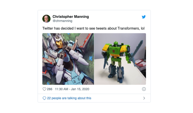
???? If you have been developing machine learning algorithms for processing sequential data — such as text in language processing, speech signals, or videos — you probably have heard about or used the Transformer model, and you probably know it’s different from the one that twitter thinks:
???????? Recently, Google introduced the Reformer architecture, a Transformer model designed to efficiently handle processing very long sequences of data (e.g. up to 1 million words in a language processing). Execution of Reformer requires much lower memory consumption and achieves impressive performance even when running on only a single GPU. The paper Reformer: The efficient Transformer will be presented in ICLR 2020 (and has received a near-perfect score in the reviews). Reformer model is expected to have a significant impact on the filed by going beyond language applications (e.g. music, speech, image and video generation).
???? In this post, we will try to dive into the Reformer model and try to understand it with some visual guides. Ready? ????
Why Transformer?
???? A class of tasks in NLP (e.g. machine translation, text generation, question answering) can be formulated as a sequence-to-sequence learning problem. Long short term memory (LSTM) neural networks, later equipped with an attention mechanism, were a prominent architecture used to build prediction models for such problems — e.g. in Google’s Neural Machine Translation System. However, the inherently sequential nature of recurrence in LSTMs, was the biggest obstacle in parallelization of computation over the sequence of data (in terms of speed and vanishing gradients), and as a result, those architectures could not take advantage of the context over long sequences.
???? The more recent Transformer model — introduced in the paper Attention is all you need — achieved state of the art performance in a number of tasks by getting rid of recurrence and instead introducing multi-head self-attention mechanism. The main novelty of the transformer was its capability of parallel processing, which enabled processing long sequences (with context windows of thousands of words) resulting in superior models such as the remarkable Open AI’s GPT2 language model with less training time. ???? Huggingface’s Transformers library — with over 32+ pre-trained models in 100+ languages and interoperability between TensorFlow and PyTorch — is a fantastic open-source effort for building state-of-the-art NLP systems. ???? Write with transformers and Talk to Transformers are some of the fun demos to play with. The Transformer has been used for applications beyond text as well such as generating music and images.
What’s missing from the Transformer?
????Before diving deep in the reformer, let’s review what is challenging about the transformer model. This requires some understanding of the transformer architecture itself, which we cannot go through in this post. However, if you already don’t know, Jay Alamar’s The Illustrated Transformer post is the greatest visual explanation so far, and I highly encourage reading his post before going through the rest of this post.
???? Although transformer models yield great results being used on increasingly long sequences — e.g. 11K long text examples in (Liu et al., 2018) — many of such large models can only be trained in large industrial compute platforms and even cannot be fine-tuned on a single GPU even for a single training step due to their memory requirements. For example, the full GPT-2 model consists of roughly 1.5B parameters. The number of parameters in the largest configuration reported in (Shazeer et al., 2018) exceeds 0.5B per layer, while the number of layers goes up to 64 in (Al-Rfou et al., 2018).
???? Let’s look at a simplified overview of the Transformer model:

???? If this model doesn’t look familiar or seems hard to understand, I urge you to pause here and review ➡️ The Illustrated Transformer post.
You may notice there exist some ????’s in the diagram with 3 different colors. Each of these unique ????’s represents a part of the Transformer model that the Reformer authors looked at as sources of computation and memory issues:
???? Problem 1 (Red ????): Attention computation
Computing attention on sequences of length L is O(L²) (both time and memory). Imagine what happens if we have a sequence of length 64K.
???? Problem 2 (Black ????): Large number of layers
A model with N layers consumes N-times larger memory than a single-layer model, as activations in each layer need to be stored for back-propagation.
???? Problem 3 (Green ????): Depth of feed-forward layers
The depth of intermediate feed-forward layers is often much larger than the depth of attention activations.
The Reformer model addresses the above three main sources of memory consumption in the Transformer and improves upon them in such a way that the Reformer model can handle context windows of up to 1 million words, all on a single accelerator and using only 16GB of memory.
In a nutshell, the Reformer model combines two techniques to solve the problems of attention and memory allocation: locality-sensitive-hashing (LSH) to reduce the complexity of attending over long sequences, and reversible residual layers to more efficiently use the memory available.
Below we go into further details.
???? 1. Locality sensitive hashing (LSH) Attention
???? Attention and nearest neighbors
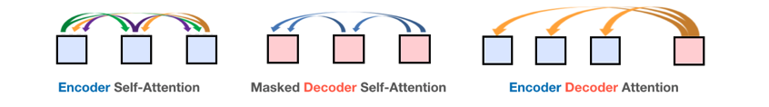
Attention in deep learning is a mechanism that enables the network to focus attentively on different parts of a the context based on their relativeness to the current timestep. There exist 3 types of attention mechanism in the transformer model as below:
The standard attention used in the Transformer is the scaled dot-product, formulated as:
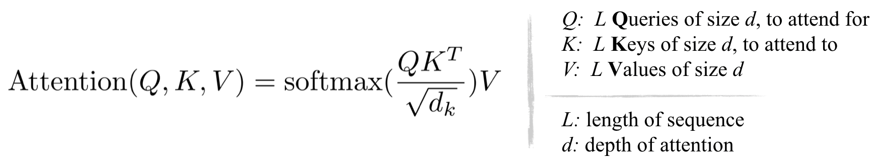
From the above equation and the figure below, it can be observed that the computational and memory cost of multiplication QKᵀ (with the shape [L, L]) are both in O(L²), which is the main memory bottleneck.

❓But is it necessary to compute and store the full matrix QKᵀ ? The answer is no, as we are only interested in softmax(QKᵀ ), which is dominated by the largest elements in a typically sparse matrix. Hence, as you can see in the above example, for each query q we only need to pay attention to the keys k that are closest to q. For example, if K is of length 64K, for each q we could only consider a small subset of the 32 or 64 closest keys. So the attention mechanism finds the nearest neighbor keys of a query but in an inefficient manner. ????Does this remind you of nearest neighbors' search?
The first novelty in the reformer comes from replacing dot-product attention with locality-sensitive hashing (LSH) to change the complexity from O(L²) to O(L log L).
???? LSH for nearest neighbors search
LSH is a well-known algorithm for an efficient and approximate way of nearest neighbors search in high dimensional datasets. The main idea behind LSH is to select hash functions such that for two points ‘p’ and ‘q’, if ‘q’ is close to ‘p’ then with good enough probability we have ‘hash(q) == hash(p)’.
The simplest way to achieve this is to keep cutting space by random hyperplanes and append sign(pᵀH) as to the hash code of each point. Let’s look at an example below:
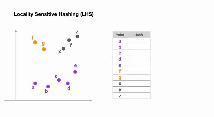
Once we find hash codes of a desired length, we divide the points into buckets based on their hash codes — in the above example, ‘a’ and ‘b’ belong to the same bucket since hash(a) == hash(b). Now the search space to find the nearest neighbors of each point reduces dramatically from the whole data set into the bucket where it belongs to.
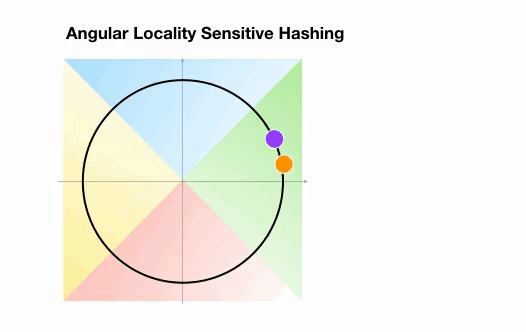
???? Angular LSH: A variant of the plain LSH algorithm, referred to as angular LSH, projects the points on a unit sphere which has been divided into predefined regions each with a distinct code. Then a series of random rotations of points define the bucket the points belong to. Let’s illustrate this through a simplified 2D example, taken from the Reformer paper:

Here we have two points that are projected onto a unit circle and rotated randomly 3 times with different angles. We can observe that they are unlikely to share the same hash bucket. In the next example, however, we see the two points that are pretty close to each other will end up sharing the same hash buckets after 3 random rotations:
???? LSH attention
Now the basic idea behind LSH attention is as follows. Looking back into the standard attention formula above, instead of computing attention over all of the vectors in Q and K matrices, we do the following:
- Find LSH hashes of Q and K matrices.
- Compute standard attention only for the k and q vectors within the same hash buckets.
Muti-round LSH attention: Repeat the above procedure a few times to increase the probability that similar items do not fall in different buckets.
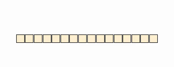
The animation below illustrates a simplified version of LSH Attention based on the figure from the paper.
???? 2. Reversible Transformer and Chunking
Now we are ready to solve the second and third issues in the Transformer, i.e. a large number of (N) encoder and decoder layers and the depth of the feedforward layers.
???? Reversible residual Network (RevNet)
Paying close attention to the encoder and decoder blocks in Fig. 2, we realize that each attention layer and feedforward layer is wrapped into a residual block (similar to what we see in Fig. 6 (left)). Residual networks(ResNets) — introduced in this paper— are powerful component used in NN architectures to help with vanishing gradient problem in deep networks (with many layers). However, memory consumption in ResNets is a bottleneck as one needs to store the activations in each layer in memory in order to calculate gradients during backpropagation. The memory cost is proportional to the number of units in the network.
To resolve this issue, the reversible residual network (RevNet) which are composed of a series of reversible blocks. In Revnet, each layer’s activations can be reconstructed exactly from the subsequent layer’s activations, which enables us to perform backpropagation without storing the activations in memory. Fig. 6. illustrates residual blocks and reversible residual blocks. Note how we can compute the inputs of the block (X₁, X₂ ) from its outputs (Y₁, Y₂).

???? Reversible Transformer
Going back to our second problem, the issue was dealing with memory requirements of N-layer Transformer network — with potentially pretty large N.
Reformer applies the RevNet idea to the Transformer by combining the attention and feed-forward layers inside the RevNet block. In Fig. 6, now F becomes an attention layer and G becomes the feed-forward layer:
Y₁ = X₁ + Attention(X₂),
Y₂= X₂+ FeedForward(Y₁)
???? Now using reversible residual layers instead of standard residuals enables storing activations only once during the training process instead of N times.
???? Chunking
The last portion of efficiency improvements in the Reformer deal with the 3rd problem, i.e. high dimensional intermediate vectors of the feed-forward layers — that can go up to 4K and higher in dimensions.
Due to the fact that computations in feed-forward layers are independent across positions in a sequence, the computations for the forward and backward passes as well as the reverse computation can be all split into chunks. For example, for the forward pass we will have:

Chunking in the forward pass computation [Image is taken from the Reformer paper]
???? Experimental Results
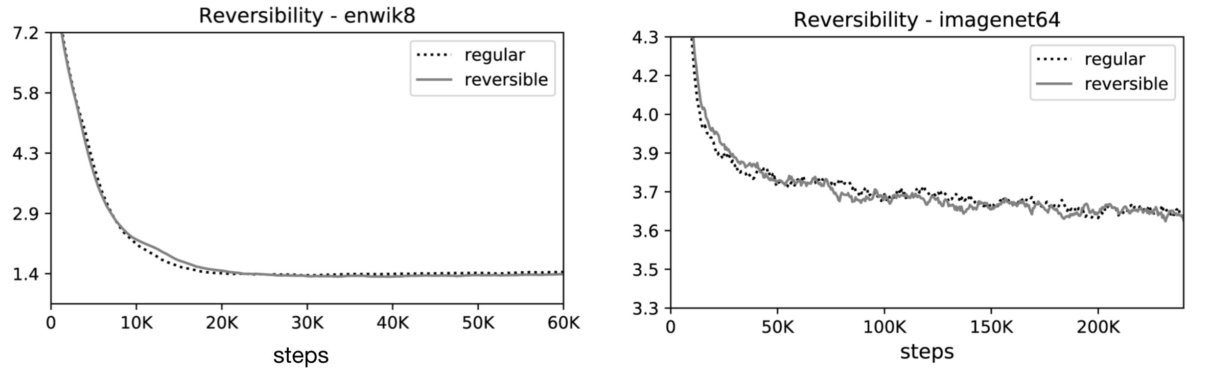
The authors conducted experiments on two tasks: the image generation task imagenet64 (with sequences of length 12K) and the text task enwik8 (with sequences of length 64K), and evaluated the effect of reversible Transformer and LSH hashing on the memory, accuracy, and speed.
???? Reversible Transformer matches baseline: Their experiment results showed that the reversible Transformer saves memory without sacrificing accuracy:
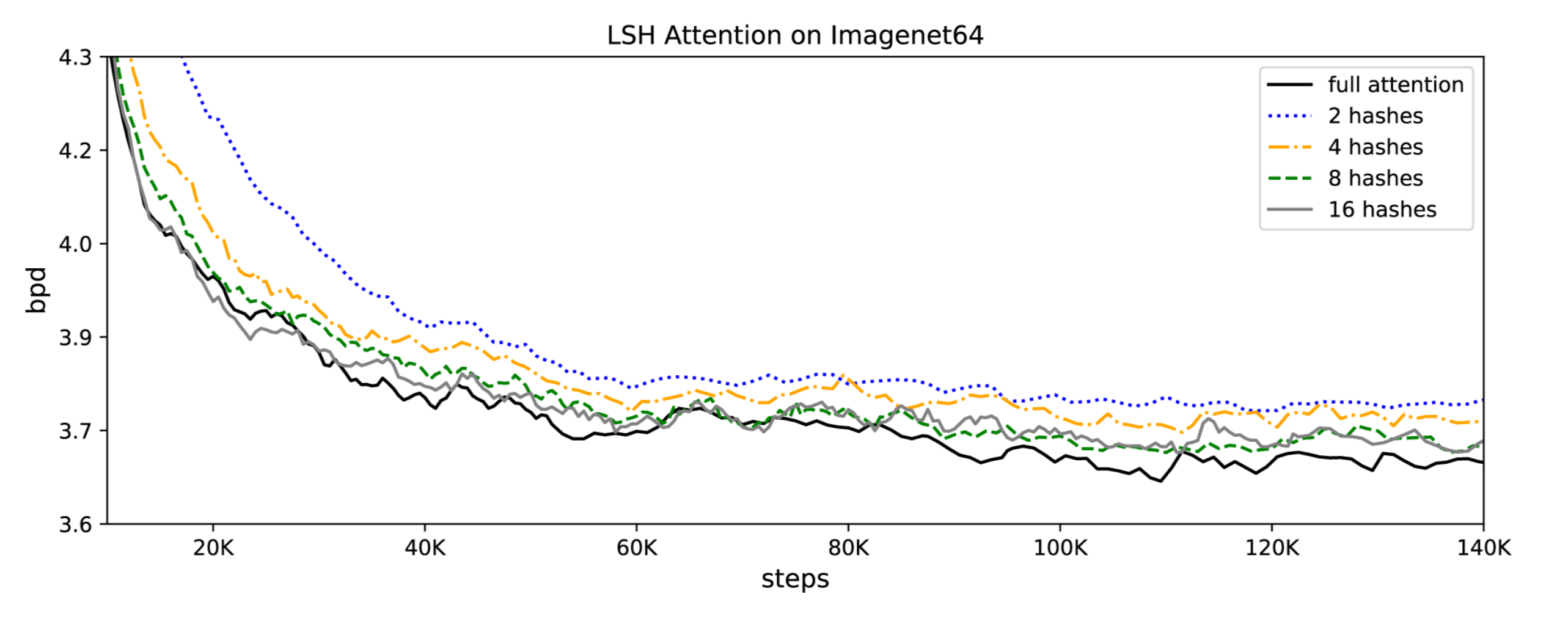
???? LSH attention matches baseline:????Note that as LSH attention is an approximation of full attention, its accuracy improves as the hash value increases. When the hash value is 8, LSH attention is almost equivalent to full attention:
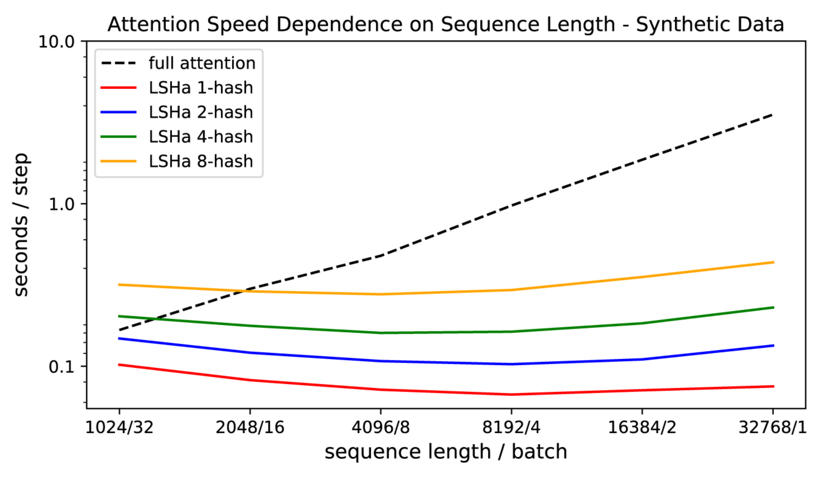
???? They also demonstrated that the conventional attention slows down as the sequence length increases, while LSH attention speed remains steady, and it runs on sequences of length ~100K at usual speed on 8GB GPUs:
The final Reformer model performed similarly compared to the Transformer model, but showed higher storage efficiency and faster speed on long sequences.
???? Trax: Code and examples
???? The code for the Reformer has been released as part of the new Trax library. Trax is a modular deep learning training and inference library which is aimed to allow you to understand deep learning from scratch. The Reformer code includes several examples that you can train and infer on image generation and text generation tasks.
???? Acknowledgment
I would like to thank Łukasz Kaiser for his vivid presentation of the Reformer and providing supplementary material. I would also like to thank Abraham Kang for his deep review and constructive feedback.
???? References and related links:
Reformer: The Efficient Transformer
Understanding sequential data - such as language, music or videos - is a challenging task, especially when there is…
Transformer: A Novel Neural Network Architecture for Language Understanding
Neural networks, in particular recurrent neural networks (RNNs), are now at the core of the leading approaches to…
- Reformer: The efficient Transformer
- Google/Trax deep learning library
- The Illustrated Transformer
- Huggingface/Transformers NLP library
- Attention is all you need
- Open AI’s GPT2 language model
- Write with transformers
- Talk to Transformers
- Google’s Neural Machine Translation System
Bio: Alireza Dirafzoon (Github) is a machine learning enthusiast. He is into conversational AI, and was previously in VR/AR, Robotics.
Original. Reposted with permission.
Related:
- Intent Recognition with BERT using Keras and TensorFlow 2
- Generating English Pronoun Questions Using Neural Coreference Resolution
- Microsoft Open Sources Jericho to Train Reinforcement Learning Using Linguistic Games