Machine Learning Over Encrypted Data
This blog outlines a solution to the Kaggle Titanic challenge that employs Privacy-Preserving Machine Learning (PPML) using the Concrete-ML open-source toolkit.

This blog introduces a Privacy-Preserving Machine Learning (PPML) solution to the Titanic challenge found on Kaggle using the Concrete-ML open-source toolkit. Its main ambition is to show that Fully Homomorphic Encryption (FHE) can be used for protecting data when using a Machine Learning model to predict outcomes without degrading its performance. In this example, an XGBoost classifier model will be considered as it achieves near state-of-the-art accuracy.
The Competition
Kaggle is an online community that lets anyone build and share projects around Machine Learning and Data Science. It offers data sets, courses, examples and competitions for free to any data scientists willing to discover or improve their knowledge of the field. Its simplicity of use makes it one of the most popular platforms amongst the ML community.
Additionally, Kaggle provides several tutorials with different difficulty levels for new beginners to start manipulating basic data science tools on a real-life example. Among those tutorials can be found the Titanic competition. It introduces a binary classification problem by using a simple data set of passengers traveling during the tragic Titanic shipwreck.
The Jupyter Notebook sent by the Concrete-ML team for this competition can be found here. It has been created with the help of several other publicly available notebooks in order to offer clear guidelines along with efficient results.
Preparation
Before being able to build the model, some preparation steps are required.
Package requirements
Concrete-ML is a Python package, the code is therefore made using this programming language. A few additional packages are required, including the Pandas framework used for pre-processing the data as well as some scikit-learn cross-validation tools.
import numpy as np
import pandas as pd
from sklearn.model_selection import GridSearchCV, ShuffleSplit
from xgboost import XGBClassifier
from concrete.ml.sklearn import XGBClassifier as ConcreteXGBClassifier
Clean the data
Both training and test data sets are given in the Kaggle platform. Once this is done, let’s load the data and extract the target IDs.
train_data = pd.read_csv("./local_datasets/titanic/train.csv")
test_data = pd.read_csv("./local_datasets/titanic/test.csv")
datasets = [train_data, test_data]
test_ids = test_data["PassengerId"]
Here’s what the data looks like:
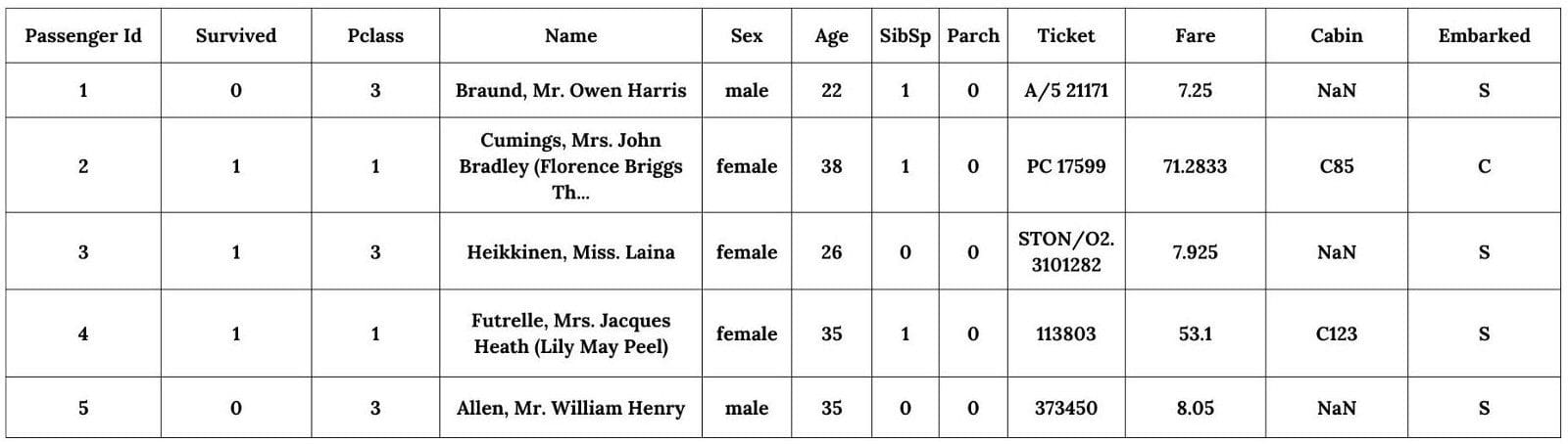
Several statements can be made :
- The target variable is the Survived variable.
- Some variables are numerical, such as PassengerID, Pclass, SbSp, Parch or Fare
- Some variables are categorical (non-numerical), such as Name, Sex, Ticket, Cabin or Embarked
A first pre-processing step is to remove the PassengerId and Ticket variables as they seem to be random identifiers that have no impact on their survival. Additionally, we can notice that some values are missing in the Cabin variable. We must therefore further investigate this observation by printing the total amounts of missing values for each variable.
print(train_data.isnull().sum())
print(test_data.isnull().sum())
This outputs the following results.
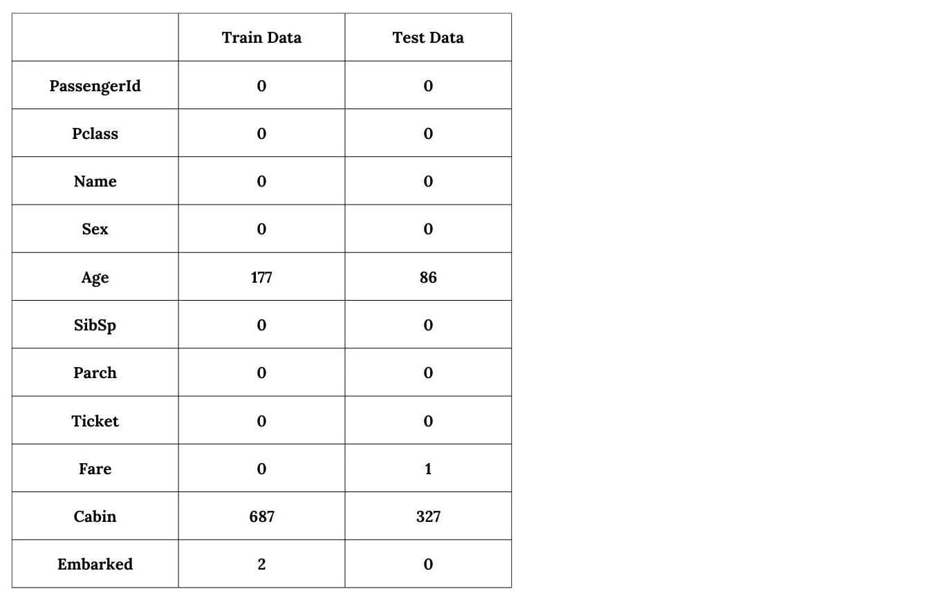
It seems that four variables are incomplete, Cabin, Age, Embarked and Fare. However, the Cabin one seems to be missing quite more data than the others:
for incomp_var in train_data.columns:

  missing_val = pd.concat(datasets)[incomp_var].isnull().sum()

  if missing_val > 0 and incomp_var != "Survived":

      total_val = pd.concat(datasets).shape[0]

      print(

         f"Percentage of missing values in {incomp_var}: "

   f"{missing_val/total_val*100:.1f}%"

      )
Percentage of missing values in Cabin: 77.5%
Percentage of missing values in Age: 20.1%
Percentage of missing values in Embarked: 0.2%
Percentage of missing values in Fare: 0.1%
Since the Cabin variable misses more than 2/3 of its values, it also might not be appropriate to keep it. We therefore drop those variables from both data sets.
drop_column = ["PassengerId", "Ticket", “Cabin”]
for dataset in datasets:
  dataset.drop(drop_column, axis=1, inplace=True)
Regarding the three other variables that witness missing values, removing them could mean losing a lot of relevant information that might help the model predicting the passengers’ survival. This is mostly true for the Age variable since more than 20% of its values are lacking. Alternative techniques can thus be used to fill in these incomplete variables. Since both Age and Fare are numerical, missing values can be replaced by the median of the available ones. For the Embarked variable, which is categorical, we use the most common value as the substitute.
for dataset in datasets:

  dataset.Age.fillna(dataset.Age.median(), inplace=True)

  dataset.Embarked.fillna(dataset.Embarked.mode()[0], inplace=True)

  dataset.Fare.fillna(dataset.Fare.median(), inplace=True)
Engineer new features
Furthermore, we can manually create new variables from already existing ones in order to help the model interpret some behaviors for better predictions. Among all available possibilities, four new features were selected:
- FamilySize: The size of the family the individual was traveling with, with 1 being someone that traveled alone.
- IsAlone: A boolean variable stating if the individual was traveling alone (1) or not (0). This might help the model to emphasize on this idea of traveling with relatives or not.
- Title: The individual's title (Mr, Mrs, ...), often indicating a certain social status.
- Farebin and AgeBin: Binned version of the Fare and Age variables. It groups values together, generally reducing the impact of minor observation errors.
Let’s create those new variables for both data sets.
# Function that helps generating proper bin names
def get_bin_labels(bin_name, number_of_bins):

  labels = []

  for i in range(number_of_bins):

      labels.append(bin_name + f"_{i}")

  return labels

for dataset in datasets:

  dataset["FamilySize"] = dataset.SibSp + dataset.Parch + 1

  dataset["IsAlone"] = 1

  dataset.IsAlone[dataset.FamilySize > 1] = 0

  dataset["Title"] = dataset.Name.str.extract(
r" ([A-Za-z]+)\.", expand=False

  )

  dataset["FareBin"] = pd.qcut(
dataset.Fare, 4, labels=get_bin_labels("FareBin", 4)

  )

  dataset["AgeBin"] = pd.cut(
dataset.Age.astype(int), 5, labels=get_bin_labels("AgeBin", 5)

  )


  # Removing outdated variables

  drop_column = ["Name", "SibSp", "Parch", "Fare", "Age"]

  dataset.drop(drop_column, axis=1, inplace=True)
Additionally, printing the different titles found within the data sets shows that only a few of them represent most of the individuals.
data = pd.concat(datasets)
titles = data.Title.value_counts()
print(titles)
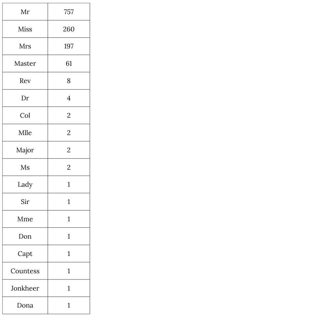
In order to prevent the model from becoming overly specific, all the "uncommon" titles are grouped together into a new “Rare” variable.
uncommon_titles = titles[titles < 10].index
for dataset in datasets:
  dataset.Title.replace(uncommon_titles, "Rare", inplace=True)
Apply dummification
Finally, we can "dummify" the remaining categorical variables. Dummification is a common technique of transforming categorical (non-numerical) data into numerical data without having to map values or consider any order between each of them. The idea is to take all the different values found in a variable and create a new associated binary variable.
For example, the "Embarked" variable has three categorical values, "S", "C" and "Q". Dummifying the data will create three new variables, "Embarked_S", "Embarked_C" and "Embarked_Q". Then, the value of "Embarked_S" (resp. "Embarked_C" and "Embarked_Q") is set to 1 for each data point initially labeled with "S" (resp. "C" and "Q") in the "Embarked" variable, and 0 if not.
categorical_features = train_data.select_dtypes(exclude=np.number).columns
x_train = pd.get_dummies(train_data, prefix=categorical_features)
x_test = pd.get_dummies(test_data, prefix=categorical_features)
x_test = x_test.to_numpy()
We then split the target variable from the others, a necessary step before training.
target = "Survived"
x_train = x_train.drop(columns=[target])
x_train = x_train.to_numpy()
y_train = train_data[target].to_numpy()
Building the model
Training with XGBoost
Let's first build a classifier model using XGBoost. Since several parameters have to be fixed beforehand, we use scikit-learn's GridSearchCV method to perform cross validation in order to maximize our chance to find the best ones. The given ranges are voluntarily small in order to keep the FHE execution time per inference relatively low (below 10 seconds). In fact, we found out that, in this particular Titanic example, models with larger numbers of estimators or maximum depth don't score a much better accuracy. We then fit this model using the training sets.
cv = ShuffleSplit(n_splits=5, test_size=0.3, random_state=0)
param_grid = {

  "max_depth": list(range(1, 5)),

  "n_estimators": list(range(1, 5)),

  "learning_rate": [0.01, 0.1, 1],
}
model = GridSearchCV(

  XGBClassifier(), param_grid, cv=cv, scoring="roc_auc"
)
model.fit(x_train, y_train)
Training with Concrete-ML
Now, let's do the same using Concrete-ML's XGBClassifier method.
In order to do so, we need to specify the number of bits over which inputs, outputs and weights will be quantized. This value can influence the precision of the model as well as its inference running time, and therefore can lead the grid-search cross-validation to find a different set of parameters. In our case, setting this value to 2 bits outputs an excellent accuracy score while running faster.
param_grid["n_bits"] = [2]
x_train = x_train.astype(np.float32)
concrete_model = GridSearchCV(

  ConcreteXGBClassifier(), param_grid, cv=cv, scoring="roc_auc"
)
concrete_model.fit(x_train, y_train)
The Concrete-ML API has been thought to be as close as most common Machine Learning and Deep Learning Python libraries in order to make its use as easy as possible. Additionally, it enables any data scientists to use Zama’s technology without the need of any prior knowledge on cryptography. Building and fitting a FHE-compatible model therefore becomes very intuitive and convenient for anyone that is used to common Data Science workflows such as scikit-learn tools. In fact, those observations remain valid regarding the prediction process, with only a few additional steps to consider.
Predicting the Outcomes
Let’s first compute the predictions in clear using the XGBoost model.
clear_predictions = model.predict(x_test)
Besides, it is also possible to compute the predictions in clear using the Concrete-ML model. This will essentially execute the library’s XGBoost version of the model considering the quantization process. No FHE related computations are dealt with here.
clear_quantized_predictions = concrete_model.predict(x_test)
In order to do the same using FHE, an additional compilation step is needed. By giving it a subset of the input data used for representing the reachable range of values, the compile method builds an appropriate FHE circuit that will then be executed during the prediction. Note that the execute_in_fhe parameter also needs to be set to True.
fhe_circuit = concrete_model.best_estimator_.compile(x_train[:100])
fhe_predictions = concrete_model.best_estimator_.predict(

  x_test, execute_in_fhe=True
)
Using a machine with 8 11th Gen Intel® Core™ i5-1135G7 processors of 2.40GHz (4 cores, 2 threads each), the average execution time per inference lies between 2 and 3 seconds. This does not include the key generation time, which happens only once before all predictions are made and reaches no more than 12 seconds.
Additionally, FHE computations are expected to be exact. This means that the model executed in FHE results in the same predictions as the Concrete-ML one, which is executed in clear and only considers quantization.
number_of_equal_preds = np.sum(

  fhe_predictions == clear_quantized_predictions
)
pred_similarity = number_of_equal_preds / len(clear_predictions) * 100
print(

  "Prediction similarity between both Concrete-ML models"

  f"(quantized clear and FHE): {pred_similarity:.2f}%"
)
Prediction similarity between both Concrete-ML models (quantized clear and FHE): 100.00%
However, as seen previously, the grid-search cross-validation was done separately between the XGBoost model and the Concrete-ML one. For this reason, the two models do not share the same set of hyperparameters, making their decision boundaries different.
Comparing how similar their predictions are one by one is thus irrelevant and only the final accuracy score given by the Kaggle platform should be considered to assess their performance.
Therefore, let’s save the predictions from both XGBoost and Concrete-ML models as csv files. Then, those files can be submitted in the Kaggle platform using this link. The FHE model outputs an accuracy of around 78%, which can be seen in the public leaderboard. In comparison, the XGBoost clear one scores 77%.
In fact, using the given dataset, most of the submitted notebooks do not seem to exceed 79% of accuracy. Therefore, additional pre-processing and feature engineering might help increase our current score but probably not by much.
submission = pd.DataFrame(

      {

          "PassengerId": test_ids,

          "Survived": fhe_predictions,

      }

  )

submission.to_csv("titanic_submission_fhe.csv", index=False)

submission = pd.DataFrame(

      {

          "PassengerId": test_ids,

          "Survived": clear_predictions,

      }

  )

submission.to_csv("titanic_submission_xgb_clear.csv", index=False)
Thanks for reading! Our main idea here was not only to build a predictive model that answers the question: “what sorts of people were more likely to survive?” but also to do it on encrypted data.
This was possible thanks to our Python package: Concrete-ML that aims to simplify the use of fully homomorphic encryption (FHE) for data scientists.
Roman Bredehoft is a Machine Learning Engineer at Zama.