Picking Examples to Understand Machine Learning Model
Understanding ML by combining explainability and sample picking.

Photo by Skylar Zilka on Unsplash
Evaluating model relevance does not stop at measuring its performance. For many reasons it is important to know how it ended up making such predictions. It notably favors: a better understanding of models, explaining how it works to non-data specialists, checking bias and model consistency, and debugging,…
A machine learning model can be explained using local explainability or global explainability.
In this article, we will use a complementary approach by combining explainability and sample picking.
Sample picking is a process with great added value to better understand models, their strengths and weaknesses. To explain this approach we will answer 3 questions:
Why select samples? What kind of samples would you like to analyze? What to analyze in these samples?
Local and global explainability
Before that, let us briefly recall local and global explainability notions.
The classical forms of local explainability are weight-based methods.
The prediction of a given sample is explained by decomposing the weight of each feature used in the machine learning model.
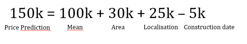
Image by Author
Global explainability consists of measuring how features are important for model prediction. This explainability is often shown as follows:
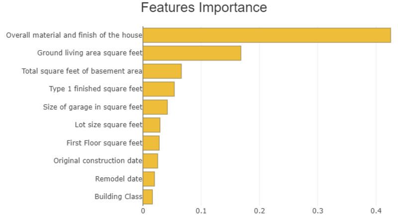
Image by Author
Now that we have quickly introduced the notions of explainability, let’s get back to the questions about picking.
To illustrate this, we use Shapash, an open-source Python library about explainability. You will find the general presentation of Shapash in this article.
The illustrations below are based on the famous Kaggle datasets: “Titanic” (for classification) and “House Prices” (for regression).
Why Select Samples?
- To explain how the model works and what are the characteristics of a single example or of a sub-population.
Let’s take for example the regression model of the price of a house based on these characteristics.
You will be able to explain to a buyer why the house is valued at this price. Or how the model estimates houses with bigger surfaces, located in a specific neighborhood, and built with wood.
- To better understand wrong predictions
This can lead to the following questions: Is the problem coming from the data quality?
If we have a very low real price and we estimate that it will be higher because the square footage of the house is high, it can question the quality of the “Surface” feature.
Could an extra feature improve the prediction?
If a real estate agent provides a textual description of what the buyer likes best. Even if this textual variable is not available at the time of prediction, we can use it to cross-reference the prediction error on samples with the buyer’s feedback.
- To illustrate correct predictions of the model
We can take examples to explain the prediction of a machine learning model. This process is easier when the most relevant examples are highlighted.
- To select samples on which to perform data quality validation or to validate the results
As a data scientist, you can have an idea of the price for some sales that the model is supposed to estimate. Exploring its local explainability would also provide you with potential reasons for rationalizing the estimation. Then you can observe the difference between your thoughts and the local explainability. Based on this you might validate or not the data quality, the prediction of the model, and the explainability.
- To study examples with experts who are familiar with the use case.
By selecting sales, you will be able to see with the real estate agent what he thinks about the price prediction and the importance of the features on the price.
What Kind of Samples Would you like to Analyze?
It is possible to analyze :
- raw model predictions
- correct predictions/errors (through the association of predictions with the known target status)
- a subset according to output probabilities of the model prediction, target to predict, values of explanatory features
Why not select random samples?
To save time and have an exhaustive vision of the different cases. Since we usually do not evaluate hundreds of samples, selecting them randomly may end up randomly picking similar samples. It would thus be possible to miss potentially interesting cases.
Data Picking: How to Easily and Reliably Pick Meaningful Examples?
Since Shapash Version 2.2.0, You can identify these samples by plotting the model probabilities for each sample provided as a function of their true label such as :
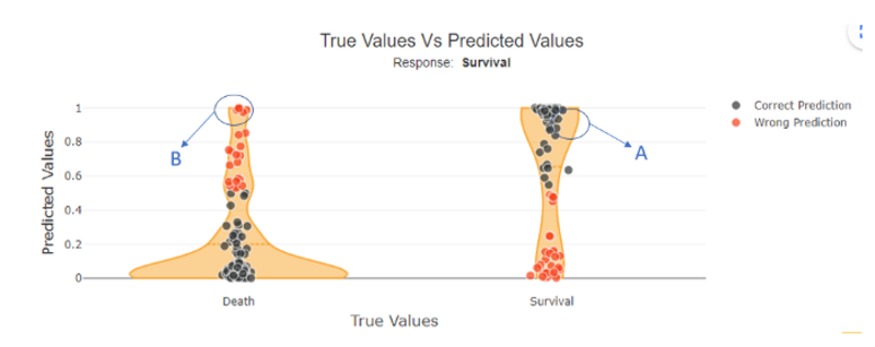
Figure 1 by Author
For binary classification with model output probabilities between 0 and 1, we could select a well-predicted class 1 sample. In this case, this class 1 displays, as expected a high probability of being in class 1 (as seen in figure 1 example A).
Oppositely, we could also select a wrongly predicted class 1 sample. Here this sample should be predicted as 0 but has a high probability of being in class 1 (as seen in figure 1 example B).
For regression, plotting the predicted values against the true values favors the direct identification and study of the best or worse predictions returned by the model.
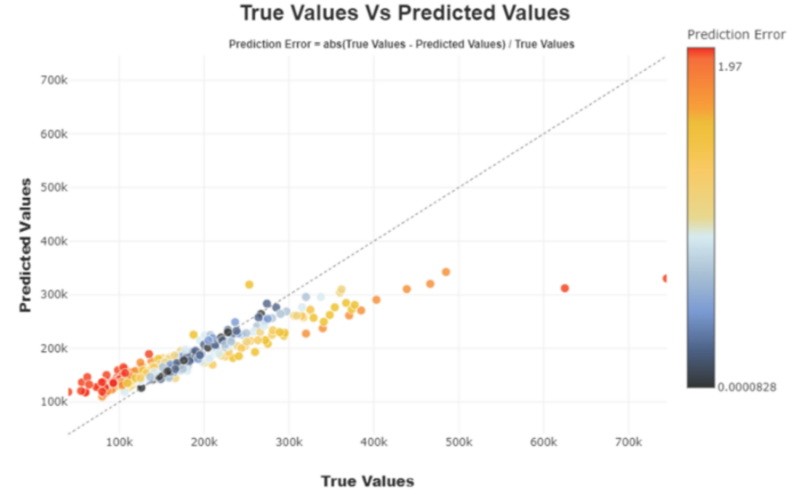
Figure 2 by Author
The selection of a subset could ease the understanding of a population’s behavior:
For binary classification, the subset could focus on all points predicted as class 1 which are in fact class 0 (i.e. the “False negative” subpopulation).
Image by Author
For regression, it can be interesting to focus on a set of well-estimated, over or under-estimated values.
You can also select a subset according to the characteristics of the explanatory features.
For example, on house price, you can select houses that have a construction date higher than 2000. Or according to the location of the house.
What to Analyze in these Samples?
- When you want to explain a single sample, it is interesting to look at its local explicability.
For example, using shapash webapp, you can select a single sample you want to analyze in the local plot:
Image by Author
The sample with the index “206” has a survival probability of 0.99, but its real label is “Death”. For this individual, the local interpretability indicates that the probability is mainly determined by the age (2 years) and by the sex (female).
Oppositely, the sample with the index “571” has a survival probability of 0.005, but its real label is “Survival”. Here again, the local interpretability indicates that the probability is mainly determined by the age (62 years) and by the sex (male).
In these 2 cases, in relation to the global functioning of the model, we understand that it is normal for the model to be wrong. For example, check that the “age” data is collected correctly, or ask whether any other data can explain that older men have survived. We can also wonder if these types of individuals are often shown in the dataset. Indeed, if only a few examples exist, the model is unable to properly learn reliable rules.
In other cases, it may help to question the data choice, data quality, or the need to collect other features.
- When you want to understand a sub-population, you can look at the global explainability of that sub-population and compare it to the global population.
For example, if you want to zoom in on the “False negative” in this app:
Image by Author
You can see if the importance of features for the subset is similar to the overall population.
For the “False negative” subpopulation, there is a decrease in the weight of the “Sex” feature on the prediction (grey vs yellow bar). This could rely on the fact that women are underrepresented in this subset. As the “Sex” feature has less impact, the other features take over. We can see that many wrong predictions rely on the variable “age”, for individuals between 20 and 30 years old.
The advantage of selecting a subset rather than a single sample is that we can generalize wrong or correct predictions, and specifically look at their global explainability in regard to the whole population.
In this example, an extra feature might help to better classify men in their twenties.
Conclusion
Picking single samples or a subset is a complementary approach that helps data scientists to understand their models.
These approaches can be used as powerful tools to explain the models to non-data technicians. It provides reliable explanations of predictions on samples to illustrate how the model works.
Sub-populations could also be described and qualified using clustering approaches.
If you use picking techniques to help understand a model, feel free to explain it in the comments!
Thomas Bouche is a Data Scientist at MAIF.