A Brief Introduction to Kalman Filters
What you can’t observe, you ought to estimate. Human evolution is based on this keen interest in measurement. But what are the quantities or phenomena which you can’t observe or measure with certainty? Learn this and more about Kalman Filter which is the most widely used algorithm to estimate a true quantity.
Introduction
Can you measure the temperature inside the core of a nuclear reactor to make sure the nuclear reaction is controlled? It certainly is too hot for any thermostat manufactured to date. So what’s our best bet? The closest one can go is to measure the temperature of a surface close to the core and estimate the temperature inside it.

Image by snowing on Freepik
Let us consider another example to internalize this concept where direct measurement of a phenomenon is not possible – can you measure the exact position of a flying object using radar technology considering variable air density, wind direction, and wind speed? What if the wind changed direction? Has the empirical error associated with the radar device been accommodated?
The environment impacts the accuracy of these measurements – if the environment isn’t controlled, you tend to get noisy readings. Therefore you would need a methodology that can filter the noise of these measurements and provide a near-accurate estimate, and the answer lies in Kalman Filter.
What is the Need for Kalman Filter?
You must be wondering your work is not directly related to the examples and the applications shared above. So, why is there a need for you to understand and learn the Kalman Filters?
Well, maybe you don’t work with nuclear reactors or radars for that matter, but what if you want to measure the position of your car moving east on a long straight road? Of course, GPS technology is what people use to measure the position of anything on this planet. But, GPS signals get impacted by a slight change in the position of the satellite, thermal noise, clouds, dust, etc.
What about the odometer, can it be used instead of GPS? Adding the odometer readings to the last known position is a simple way to know your current position. But, it turns out that the odometer readings are impacted by the size of the wheel, the tire air pressure, etc. Thus, the readings from the odometer are not that helpful to find the exact location.
You can also measure the acceleration of the car using IMU (Inertial Measurement Unit) and double integrate it to get the distance but it is accompanied by the device and mathematical errors.
Hence, there is a need for Kalman Filters that make use of the readings from all these sources to get a near-perfect estimate of position.
Understanding the Kalman Filter Algorithm
A strong grasp of concepts like state and observation is necessary to understand the internals of the Kalman filter algorithm. So, let's first define what is a state.
The state of a system “describes enough about the system to determine its future behavior in the absence of any external forces affecting the system”. For example, the actual position of the car is a state which is always hidden. So, the observation i.e. odometer reading is used to estimate this state.
With that in mind, let’s intuitively understand the Kalman Filter using an example of a car moving with a constant velocity in a straight line. Note that we can only observe the velocity through a speedometer, which can be noisy. Let’s say the velocity is 10x+10y which means 10m/s in the x-direction and 10m/s in the y-direction. Say, there is a gaussian noise added to it which the Kalman Filter doesn’t know.
Two-Step Process
A Kalman filter for estimation would broadly involve two steps:
- Prediction: It involves predicting the quantity (position of the car) and the error covariance for the next step.
- Correction: The correction step involves computing the Kalman Gain using the previous prediction along with the error between the prediction and the observation to update the estimate and the error covariance.
An overview of the process explained above is mathematically depicted in this illustration:
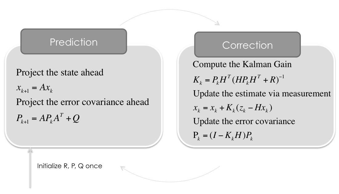
Two-Step Process by balzer82 / Kalman
The two steps are repeated for all the measurements or until the Kalman Gain stabilizes, as shown below:
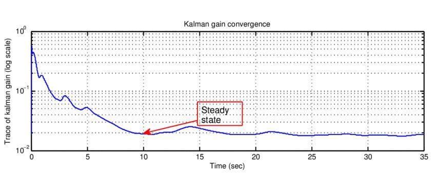
Image from ResearchGate
Estimation
The first step to solving an estimation problem is to model the problem i.e. defining the state vector that Kalman Filter would estimate. Note that we need to estimate the position as well as velocity, hence the state vector (xk) would include both. Since the distance traveled is equal to the velocity in the direction and the time elapsed, the state at time k+1 (xk+1) is defined below.
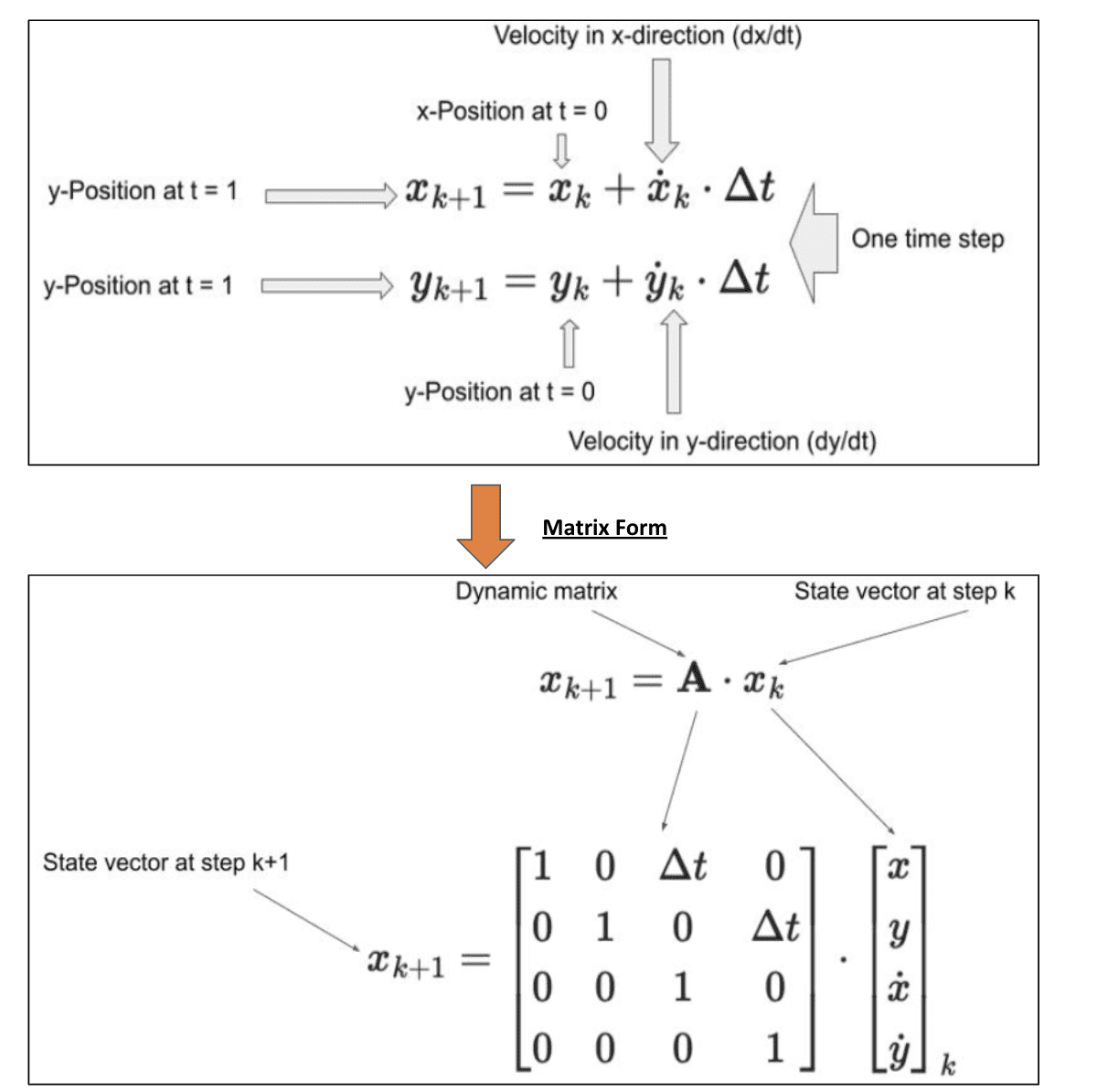
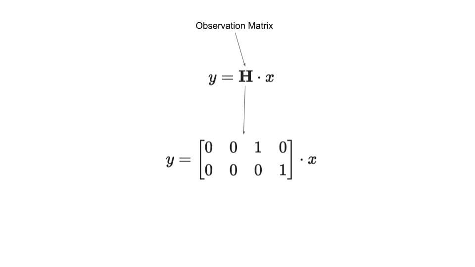
A state transition matrix A (Dynamic matrix in Kalman terms) transforms the current state of the object to the next state i.e., it defines how a state is transitioned. The second component is the observation, defined by a matrix H called the observation matrix. Because you are only observing the constant velocity and not the position, only the (1,3) and (2,4) cell of the matrix has a non-zero value.
Minimizing Noise
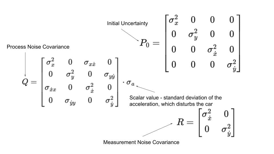
Kalman seeks to minimize noise terms which are depicted by P0, Q, and R in the two-step process. The matrix P0 captures the initial uncertainty with respect to the position and velocity. The matrix Q captures the noise to the system pertaining to environmental factors such as wind or bumpy roads, etc. The matrix R absorbs the measurement noise or errors in measurement.
Based on the iterative updates from the prediction and correction process, the Kalman Filter removes noise from a constant velocity model (the top graph) and appears like the one shown in the bottom right image. Notably, the variance in the output velocity estimate has decreased over time.
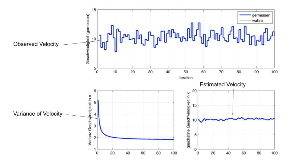
Source: The Kalman filter simply explained [Part 2]
This depicts how Kalman Filter removes noise from a constant velocity model where only one source of observation i.e. velocity is available. It works even better if there are multiple noisy sources of observation. For example, if you have the noisy odometer readings along with the velocity readings the results would have been even better.
Summary
Kalman Filter highlights the need for estimation and is used in some of the applications where noise is introduced through various sources. The article explained the internal working of the Kalman Filter through an example of 2D motion to filter this noise.
Vidhi Chugh is an AI strategist and a digital transformation leader working at the intersection of product, sciences, and engineering to build scalable machine learning systems. She is an award-winning innovation leader, an author, and an international speaker. She is on a mission to democratize machine learning and break the jargon for everyone to be a part of this transformation.