Exploratory Data Analysis Techniques for Unstructured Data
Learn how to find million-dollar insights from the data using exploratory analysis for your next data science project with Python.

Image by Author
Exploratory Data analysis is one of the crucial phases of the Machine learning development life cycle while working on any real-life data analysis project, which took almost 50-60% of the time of the whole project as the data we have to used to find insights is the raw data which has to be processed before applying Machine learning algorithms to get the best performance. This step has to include the following things:
- It involves better analyzing and summarizing data sets to understand their underlying patterns, relationships, and trends.
- It allows analysts to identify essential data features, detect anomalies or outliers, and determine the most appropriate modeling techniques for predicting future outcomes.
Let's understand the significance of EDA in Data Analytics with a story.
Understand the Importance of EDA with a Story
Once upon a time, a small firm had just started its business in the market. This firm had a group of professionals who were passionate about their role and worked in a way so that the overall firm would profit. As the firm started growing in terms of employees or users about the product it was promoting, the management team realized that they needed help understanding the need and behavior of users or customers towards the product or services the firm was offering.
To overcome this issue, they started hiring some tech professionals. Eventually, they were able to find one tech guy under the profile of Data Analyst so that they could better understand the customer data. That analyst would be able to find important information or insights from it. The analyst they hired had good hands-on experience in the same type of technology or projects where they mainly worked on exploratory data analysis.
So, for this problem, they started collecting data from multiple APIs through web scraping in an ethical manner, which includes the company website, social media handles, forums, etc. After data collection, they started with cleaning and processing the data so that they would be able to find some insights from that data. They used statistical techniques such as hypothesis testing and business intelligence tools to explore the data and uncover the hidden patterns using pattern recognition techniques.
After creating the pipeline, they observed that the company's customers were most interested in buying eco-friendly and sustainable products. The company's management launched eco-friendly and sustainable products based on these insights. So, based on these updates, the new products were liked by the customers, and eventually, the company's revenue started multiplying. Management has started realizing the importance of exploratory data analysis and hired more data analysts.
Therefore, In this article, inspired by the story mentioned above, we will understand different techniques inside the exploratory data analysis phase of the pipeline and use popular tools in this process, through which you can find million-dollar insights for your company. This article provides a comprehensive overview of EDA and its importance in data science for beginners and experienced data analysts.
Different Techniques to Implement
To understand each technique used inside EDA, we will go through one dataset and implement it using Python libraries for Data Science, such as NumPy, Pandas, Matplotlib, etc.
The dataset we will use in our analysis is Titanic Dataset, which can be downloaded from here. We will use train.csv for model training.
1. Import Necessary Libraries and Dependencies
Before implementing, let’s first import the required libraries that we are going to utilize to implement different EDA techniques, including
- NumPy for matrix manipulation,
- Pandas for data analysis, and
- Matplotlib and Seaborn for Data Visualization.
import numpy as np
import pandas as pd
import matplotlib.pyplot as plt
import seaborn as sb
2. Load and Analyze the Dataset
After importing all the required libraries, we will load the Titanic dataset using the Pandas dataframe. Then we can start performing different Data preprocessing techniques to prepare the data for further modeling and generalization.
passenger_data = pd.read_csv('titanic.csv')
passenger_data.head(5)
Output:

Fig. 1 | Image by Author
3. Get Statistical Summary
The following analysis provides us with the statistics of all the numerical columns in the data. The statistics which we can obtain from this function are:
- Count,
- Mean, and Median
- Standard Deviation
- Minimum and Maximum Values
- Different Quartiles Values
passenger_data.describe()
Output:
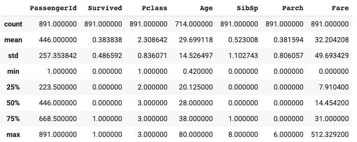
Fig. 2 | Image by Author
By interpreting the above output, we can see that there are 891 passengers with an average survival rate of 38%. The minimum and maximum value of the age columns lies between 0.42 to 80, and the average age is approximately 30 years. Also, a minimum of 50% of the passengers don't have siblings/spouses, and a minimum of 75% don't have parents/children, and the fare column varies a lot in terms of values.
Let's try to compute the survival rate by writing the code from scratch.
4. Compute the Overall Survival Rate of Passengers
To compute the overall survival rate, we first select the 'Survived' column, check the rows for which the value is one, and then count all those rows. Finally, to find the percentage, we will divide it by the total number of rows and print it.
survived_data = passenger_data[passenger_data['Survived'] == 1]
survived = survived_data.count().values[1]
survival_percent = (survived/891) * 100
print('The percentage of survived people in training data are {}'.format(survival_percent))
Output:
The percentage of survived people in training data are 38.38383838383838
5. Compute the Survival Rate by Gender and the ‘Pclass’ Column
Now, we have to find the survival rate with one of the aggregation operators wrt different columns, and we are going to use the 'gender' and 'Pclass' columns and then apply the mean function to find it and then print it.
survival_rate = passenger_data[['Pclass', 'Sex','Survived']].groupby(['Pclass', 'Sex'], as_index = False).mean().sort_values('Survived', ascending = False)
print(survival_rate)
Output:
  Pclass     Sex  Survived
0       1  female  0.968085
2       2  female  0.921053
4       3  female  0.500000
1       1    male  0.368852
3       2    male  0.157407
5       3    male  0.135447
6. Change the Data Type of Passenger Id, Survived, and Pclass to String
Since some of the columns are of different data types, we convert all those columns to a fixed data type. i.e, string.
Cols = [ 'PassengerId', 'Survived', 'Pclass' ]
for index in Cols:
     passenger_data[index] = passenger_data[index].astype(str)
passenger_data.dtypes
7. Duplicated Rows in the Dataset
While doing the data modeling, our performance can decrease if duplicated rows are present. So, it's always recommended to remove the duplicated rows.
passenger_data.loc[passenger_data.duplicated(), :]
8. Creating the Histograms to Check Data Distribution
To find the distribution of the survived columns based on the possible values of that column so that we can check the class biasness and if there are any issues, we can apply techniques such as Oversampling, undersampling, SMOTE, etc. to overcome that issue.
sb.set_style("white")
g = sb.FacetGrid(data = train[train['Age'].notna()], col = 'Survived')
g.map(plt.hist, "Age");
Output:
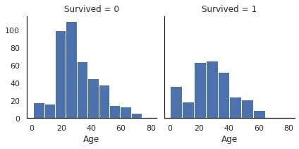
Fig. 3 | Image by Author
Now, if we compare the above two distributions then it is recommended to use the relative frequency instead of the absolute frequency by using Cumulative density function, etc. Since we have taken the example of the Age column, the histogram with absolute frequency suggests that there were many more victims than survivors in the age group of 20–30.
9. Plot Percentage of Missing Values in Age by Survival
Here we have created the pie chart to find the percentage of missing values by Survival values and then see the partition.
dt0 = train['Age'][train['Survived']=='0']
dt1 = train['Age'][train['Survived']=='1']
plt.figure(figsize = [15, 5])

plt.subplot(1, 2, 1)
age_na_pie(dt0)
plt.title('Survived: No');

plt.subplot(1, 2, 2)
age_na_pie(dt1)
plt.title('Survived: Yes');
Output:
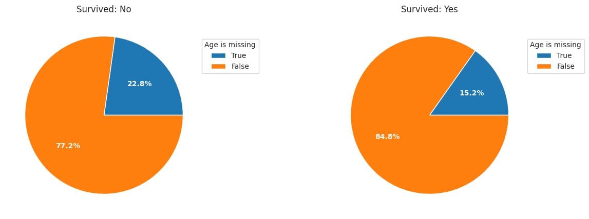
Fig. 4 | Image by Author
The pie plots show that passengers with missing ages were more likely to be victims.
10. Finding the Number of Missing Values in each Column
passenger_data.isnull().sum()
From the output, we have observed that the column "Cabin" has the maximum missing values so we will drop that column from our analysis.
11. Percentage of Null Values per column
passenger_data.isna().sum()/passenger_data.shape[0]
In age column, approximately 20% of data is missing, approximate 77% of data in Cabin Columns is missing, and 0.2 percent of data in Embarked column is missing. Our aim is to handle the missing data before modeling.
12. Drop the Cabin Column from the Dataset
Drop the cabin column, as it has many missing values.
drop_column = passenger_data.drop(labels = ['Cabin'], axis = 1)
print(drop_column)
To handle the "Age" column, firstly, we will check the data type of the age column and convert it to integer data type and then fill all the missing values in the age column with the median of the age column.
datatype = passenger_data.info('Age')
fill_values = passenger_data['Age'].fillna(int(passenger_data['Age'].median()),inplace=True)
print(fill_values)
After this, our dataset looks good regarding missing values, outliers, etc. Now, if we apply machine learning algorithms to find the patterns in the dataset and then test on the testing data, the model's performance will be more compared to data without preprocessing and exploratory data analysis or data wrangling.
Summary Insights from EDA
Here are survivors' characteristics compared to victims.
- Survivors were likely to have parents or children with them; compared to others, they had more expensive tickets.
- Children were more likely to survive than victims of all age groups.
- Passengers with missing ages were less likely to be survivors.
- Passengers with higher pclass (SES) were more likely to survive.
- Women were much more likely to survive than men.
- Passengers at Cherbourg had a higher chance of survival than Queenstown and Southampton passengers.
You can find a colab notebook here for the complete code - Colab Notebook.
Conclusion
This ends our discussion. Of course, there are many more techniques in EDA than I just covered here, which depend on the dataset we will use in our problem statement. To sum up, the EDA, knowing your data before you use it to train your model with it, is beneficial. This technique plays a crucial role in any Data Science Project, allowing our simple models to perform better when used in projects. Therefore, every aspiring Data Scientist, Data Analyst, Machine Learning Engineer, and Analytics Manager needs to know these techniques properly.
Until then, keep reading and keep learning. Feel free to contact me on Linkedin in case of any questions or suggestions.
Aryan Garg is a B.Tech. Electrical Engineering student, currently in the final year of his undergrad. His interest lies in the field of Web Development and Machine Learning. He have pursued this interest and am eager to work more in these directions.