Anomaly Detection in Predictive Maintenance with Time Series Analysis
How can we predict something we have never seen, an event that is not in the historical data? This requires a shift in the analytics perspective! Understand how to standardization the time and perform time series analysis on sensory data.
By Rosaria Silipo
The Newest Challenge
Most of the data science use cases are relatively well established by now: a goal is defined, a target class is selected, a model is trained to recognize/predict the target, and the same model is applied to new never-seen-before productive data.
The newest challengelies in predicting the “unknown”, i.e. an anomaly. An anomaly is an event that is not part of the system’s past; an event that cannot be found in the system’s historical data. In the case of network data, an anomaly can be an intrusion, in medicine a sudden pathological status, in sales or credit card businesses a fraudulent payment, and, finally, in machinery a mechanical piece breakdown.
In the manufacturing industry, the goal is to keep a mechanical pieceworking as long as possible–mechanical pieces are expensive – and at the same time to predict its breaking point before it actually occurs–a machine breakoften triggers a chain reaction of expensive damages. Therefore, a high value is usually associated with the early discovery, warning, prediction, and/or prevention of anomalies.Specifically, the prediction of “unknown” disruptive events in the field of mechanical maintenance takes the name of “anomaly detection”.
The problem here is: how can we predict something we have never seen, an event that is not in the historical data? This requires a shift in the analytics perspective! If data describing normal functioning is what we have, then normal functioning we will predict!
Pre-processing: Standardization and Time Alignment
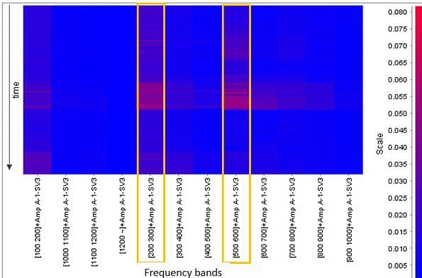
For this project, we worked on FFT pre-processed sensor data from 28 sensors monitoring a working rotor. The FFT transform produces a matrix of spectral amplitudes for a time segment anda frequency value.
In order to standardize the time and frequency references, frequency values were binned into 100Hz-wide bands and time values were binned into dates. The FFT spectral amplitudes were then averaged acrosseach date and each frequency bin.Cells in the final FFT matrix refer to one single date and one single frequency band for a single sensor.Considering all sensors, we get 313 FFT spectral amplitude columns in total.
After this standardization task, a time alignment was performed, inserting missing cell values where no date was available. The final FFT matrix has dates on one axis, frequency bins on the other axis, and average spectral amplitudes as cell values, with occasional missing values.
That is for each sensor and for each frequency band, we get a time series of spectral amplitude values evolving over time.
Predicting Anomalies using Time Series Analysis
As our data set contains only data that describe the normal functioning of the rotor, we use these data to predict anomaly-free measure values and we measure whether such a prediction is good enough. If it is not, we can assume we are out of the range of “normal functioning” and we can trigger an inspection alarm.
Themore accuratethe prediction model for the normal functioning signal, the more precise and more robust the consequent alarm is that is triggered. With this goal, an auto-regressive (AR) model is trained on an anomaly-free time window using 10 past history sampleson each one of the 313 spectral amplitude time series.
Some boundaries of normal functioning values are then defined around the average prediction error observed in training. During deployment on new data, if the prediction error diverts from these boundaries, an alarm is triggered to alert that is time to inspect the machinery.
Deployment and Optimization
Because the AR models have been trained over a time window of normal functioning, they can predict the next measure only for a correctly working rotor. Most models will actually fail at predicting the next measure, if the rotor functioning has already started to change.
During deployment:
- the AR models are applied toproductive data to predict the next value
- the distance error is calculated between the original next value and the predicted next value
- this distance erroris compared with the boundary defined on the training window:
IF (distance *distance) > boundaryTHEN alarm = distance
This generates 313 “alarm” time series. Due to temporary inabilities of the models to match the real values with the predictions, random spikes can arise in the “alarm” time series. Thus, in order to make the alarm system more reliable, we use a two-level structure: this first alarm, the one defined above, is merely a warning signal and is processed again to produce a more accurate second level alarm signal. Using a Moving Aggregation node, the moving averages are calculated on a backward window of 21 samples of the level 1 alarm (warning) signals. This moving average operation smooths out all short random spikes in the level 1 alarm time series, retaining only the ones that persist over time.
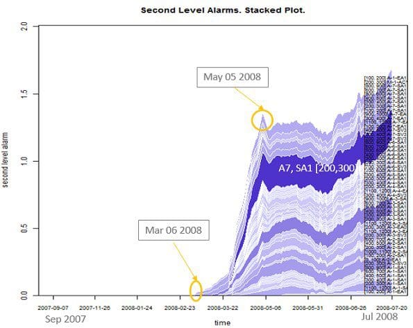
Figure 2 shows a stacked plot of the 2nd level alarm time series. Here the early signs of the rotor breakdown – which occurred on July 22 2008 – can be tracked back as early as March 2008 ‒ if using a sensitive threshold, or as early as May 2008 ‒ if using a threshold that is not so sensitive.
Summing up all 313 alarm values across all frequency bands and referring to the same date naturally improves the system performance, in terms of both specificity and sensitivity. An optimization loop, maximizing the trigger accuracy, can also help to define the optimal threshold on the 2nd level alarm time series.
Once the models and alarm criteria are in place, the final part of the deployment workflowneeds to take action, if needed. Many possible consequent actions can be started and controlled from within a KNIME workflow through a specific node or just a general REST interface: e.g. howling sirens, system switch-off, or just sending an email to the employeewho is in charge of mechanical checkups. In our deployment workflow, the designed action consists of sending an email. The 2ndlevel alarm value is then transformed into a flow variable that triggers the output port of a CASE Switch node connected to a Send Email node.
Whitepapers and Workflows
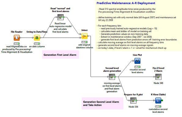
The final deployment workflow, named “Time Series AR Deployment”, is shown in Figure 3. There you can see the metanode that generates the 1st level alarms, the metanode that generates the 2nd level alarms, and the metanode that takes action named “Fire if Level 2 Alarm”. Workflows and data used for this study can be found on the KNIME EXAMPLES Server under 050_Applications/050017_AnomalyDetection/Time Series Analysis.
The whitepapers, describing the full details of this implementation, can be downloaded from for the pre-processing part and from for the time series analysis part.
For this and some more talks about Internet of Things applications, just visit us at the KNIME Spring Summit in Berlin on February 24-26 2016.
This blog post is an extraction of an article posted on the KNIME blog on Nov 30 2015: original.
Bio: Rosaria Silipo has been a researcher in applications of Data Mining and Machine Learning for over a decade. Application fields include biomedical systems and data analysis, financial time series (including risk analysis), and automatic speech processing.
Related: