Adversarial Validation, Explained

By Zygmunt Zając, FastML.

Many data science competitions suffer from a test set being markedly different from a training set (a violation of the “identically distributed” assumption). It is then difficult to make a representative validation set. We propose a method for selecting training examples most similar to test examples and using them as a validation set. The core of this idea is training a probabilistic classifier to distinguish train/test examples.

In part one, we inspect the ideal case: training and testing examples coming from the same distribution, so that the validation error should give good estimation of the test error and classifier should generalize well to unseen test examples.

In such situation, if we attempted to train a classifier to distinguish training examples from test examples, it would perform no better than random. This would correspond to ROC AUC of 0.5.

Does it happen in reality? It does, for example in the Santander Customer Satisfaction competition at Kaggle.

We start by setting the labels according to the task. It’s as easy as:

train = pd.read_csv( 'data/train.csv' )
test = pd.read_csv( 'data/test.csv' )

train['TARGET'] = 1
test['TARGET'] = 0

Then we concatenate both frames and shuffle the examples:

data = pd.concat(( train, test ))

data = data.iloc[ np.random.permutation(len( data )) ]
data.reset_index( drop = True, inplace = True )

x = data.drop( [ 'TARGET', 'ID' ], axis = 1 )
y = data.TARGET

Finally we create a new train/test split:

train_examples = 100000

x_train = x[:train_examples]
x_test = x[train_examples:]
y_train = y[:train_examples]
y_test = y[train_examples:]

Come to think of it, there’s a shorter way (no need to shuffle examples beforehand, too):

from sklearn.cross_validation import train_test_split

x_train, x_test, y_train, y_test = train_test_split( x, y, train_size = train_examples )

Now we’re ready to train and evaluate. Here are the scores:

# logistic regression / AUC: 49.82%
# random forest, 10 trees / AUC: 50.05%
# random forest, 100 trees / AUC: 49.95%

Train and test are like two peas in a pod, like Tweedledum and Tweedledee - indistinguishable to our models.

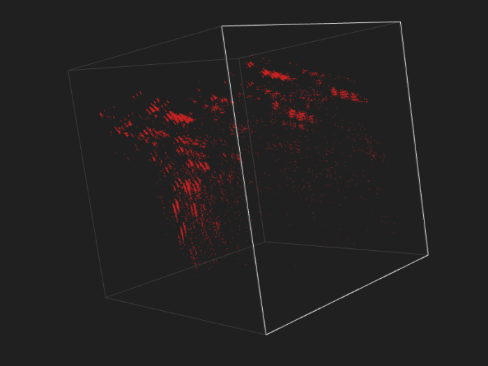
Below is a 3D interactive visualization of the combined train and test sets, in red and turquoise. They very much overlap. Click the image to view the interactive version (might take a while to load, the data file is ~8MB).

UPDATE: The hosting provider which shall remain unnamed has taken down the account with visualizations. We plan to re-create them on Cubert. In the meantime, you can do so yourself.

UPDATE: It’s a-live! Now you can create 3D visualizations of your own data sets. Visit cubert.fastml.com and upload a CSV or libsvm-formatted file.

Let’s see if validation scores translate into leaderboard scores, then. We train and validate logistic regression and a random forest. LR gets 58.30% AUC, RF 75.32% (subject to randomness).

On the private leaderboard LR scores 61.47% and RF 74.37%. These numbers correspond pretty well to the validation results.

The code is available at GitHub.

Originals: Part 1. Part 2. Reposted with permission.