Propensity Score Matching in R
Propensity scores are an alternative method to estimate the effect of receiving treatment when random assignment of treatments to subjects is not feasible.
The concept of Propensity score matching (PSM) was first introduced by Rosenbaum and Rubin (1983) in a paper entitled “The Central Role of the Propensity Score in Observational Studies for Casual Effects.”
Statistically it means...
Propensity scores are an alternative method to estimate the effect of receiving treatment when random assignment of treatments to subjects is not feasible. PSM refers to the pairing of treatment and control units with similar values on the propensity score; and possibly other covariates (the characteristics of participants); and the discarding of all unmatched units.
What is PSM in simple terms...
PSM is done on observational studies. It is done to remove the selection bias between the treatment and the control groups.
For example say a researcher wants to test the effect of a drug on lab rats. He divides the rats in two groups and tests the effects of the drug in one of the groups, which is the treatment group. The other group is known as the control group. As it is an experiment everything is controlled by the experimenter, like all these rats are genetically the same and grow up in the same environment, so he knows that any differences between them will be solely due to the drug that he has given them.
However this cannot be done with people because people are different from each other, they come in different shapes and sizes, ages, ethnicities, etc., However, at the same time people aren't so different that we can't find any similarities between them. This is when we can use propensity score matching.
To give an example, if a marketer wants to observe the effect of a marketing campaign on the buyers; to judge if the campaign is the only reason which influenced them to buy; he cannot deduce this as he does not know whether the people who participated in the campaign are equivalent to the people who did not participate in the campaign. There might be other influential factors that led the buyers to buy and it might not be the effect of the campaign at all. In that case he can go for a propensity score matching estimation to observe how much impact the campaign had on the buyers/non-buyers.
PSM using R...
I will now demonstrate a simple program on how to do Propensity Score matching in R, with the use of two packages: Tableone and MatchIt.
The dataset...
#Reading the raw data
> Data <- read.csv("Campaign_Data.csv", header = TRUE)
> dim(Data)
[1] 1000    4
The dataset contains randomly simulated 1000 records of people with their demographic profiles, age and income, the Ad_Campaign_Response, whether they have responded to the campaign or not , 1 = Responded and 0 = Not Responded, and the Bought column, 1 = Purchased and 0 = Not Purchased.
# To view the first few records in the dataset
> head(Data)
  Age  Income  Ad_Campaign_Response   Bought
1  41    107                    1       1
2  56     75                    0      0
3  50     88                    0       0
4  22     94                    1       0
5  51     74                    1       0
6  45     51                    1       1
The Treatment and Control Population...
# The treatment population
> Treats <- subset(Data,  Ad_Campaign_Response == 1)
> colMeans(Treats)
                 Age               Income  Ad_Campaign_Response        Bought
          45.7500000           79.2772277            1.0000000             0.8391089

# The control population
> Control <- subset(Data, Ad_Campaign_Response == 0)
> colMeans(Control)
                 Age               Income  Ad_Campaign_Response                  Bought
          45.0755034           79.4832215            0.0000000             0.1107383

> dim(Treats)
[1] 404   4
> dim(Control)
[1] 596   4

#Here we see we have 404 treated records and 596 control records.
If we want to find out the real impact of the campaign on the purchase
> model_1 <- lm(Bought ~ Ad_Campaign_Response + Age + Income,data=Data)
> model_1

Call:
lm(formula = Bought ~ Ad_Campaign_Response + Age + Income, data = Data)

Coefficients:
         (Intercept)  Ad_Campaign_Response                   Age                Income
           0.2201474             0.7291988             -0.0014048            -0.0005798

> Effect <- model_1$coeff[2]
> Effect
Ad_Campaign_Response
           0.7291988
The model above shows that the ad campaign had a 72.9% effect on the purchase.
The Propensity Scores Model...
Now let’s prepare a Logistic Regression model to estimate the propensity scores. That is, the probability of responding to the ad campaign.
> pscores.model <- glm(Ad_Campaign_Response ~ Age + Income,family = binomial("logit"),data = Data)
> summary(pscores.model)
Call:
glm(formula = Ad_Campaign_Response ~ Age + Income, family = binomial("logit"),
data = Data)
Deviance Residuals:
Min 1Q Median 3Q Max
-1.1095 -1.0208 -0.9926 1.3373 1.4521
Coefficients:
Estimate Std. Error z value Pr(>|z|)
(Intercept) -0.6332998 0.4505631 -1.406 0.160
Age 0.0065209 0.0063705 1.024 0.306
Income -0.0006507 0.0041133 -0.158 0.874
(Dispersion parameter for binomial family taken to be 1)
Null deviance: 1349.2 on 999 degrees of freedom
Residual deviance: 1348.1 on 997 degrees of freedom
AIC: 1354.1
Number of Fisher Scoring iterations: 4
> Propensity_scores <- pscores.model
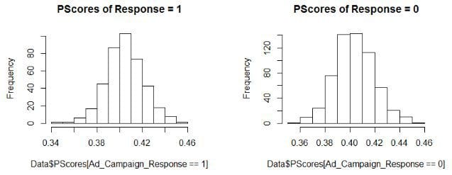
> Data$PScores <- pscores.model$fitted.values
> hist(Data$PScores[Ad_Campaign_Response==1],main = "PScores of Response = 1")
> hist(Data$PScores[Ad_Campaign_Response==0], ,main = "PScores of Response = 0")
Creating a Tableone pre-matching table...
#covariates we are using
>xvars <- c("Age", "Income")
>library(tableone)
> table1 <- CreateTableOne(vars = xvars,strata = "Ad_Campaign_Response",data = Data, test = FALSE)
We will use the tableone package to summarize the data using the covariates that we stored in xvars. We are going to stratify the response variable, i.e., we will check the balance in the dataset among the people who responded (treatment group) and who did not respond (control group) to the campaign. The ‘test = False’ states that we don’t require a significance test; instead we just want to see the mean and standard deviation of the covariates in the results.
Then we are going to print the statistics and also see the Standardized Mean Differences (SMD) in the variables.
> print(table1, smd = TRUE)
                    Stratified by Ad_Campaign_Response
                             0              1              SMD
  n                            596            404
  Age (mean (sd))       45.08 (10.02)  45.75 (10.33)   0.066
  Income (mean (sd))  79.48 (15.80)  79.28 (15.55)   0.013
Here we see the summary statistics of the covariates, we can see that in the control group there are 596 subjects and in the treatment group there are 404 subjects. It also shows the mean and standard deviations of these variables.
In the last column we can see the SMD, here we should be careful about SMDs which are greater than 0.1 because those are the variables which shows imbalance in the dataset and that is where we actually need to do propensity score matching.
In our example here, as it is a simulated dataset of just 1000 records and containing only 2 covariates we don’t see any imbalance but we will still go ahead with the matching and see the difference in the results.