Practical Hyperparameter Optimization
An introduction on how to fine-tune Machine and Deep Learning models using techniques such as: Random Search, Automated Hyperparameter Tuning and Artificial Neural Networks Tuning.
By Pier Paolo Ippolito, The University of Southampton
Introduction
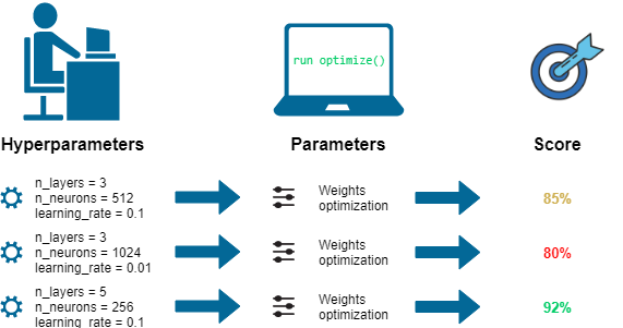
Machine Learning models are composed of two different types of parameters:
- Hyperparameters = are all the parameters which can be arbitrarily set by the user before starting training (eg. number of estimators in Random Forest).
- Model parameters = are instead learned during the model training (eg. weights in Neural Networks, Linear Regression).
The model parameters define how to use input data to get the desired output and are learned at training time. Instead, Hyperparameters determine how our model is structured in the first place.
Machine Learning models tuning is a type of optimization problem. We have a set of hyperparameters and we aim to find the right combination of their values which can help us to find either the minimum (eg. loss) or the maximum (eg. accuracy) of a function (Figure 1).
This can be particularly important when comparing how different Machine Learning models performs on a dataset. In fact, it would be unfair for example to compare an SVM model with the best Hyperparameters against a Random Forest model which has not been optimized.
In this post, the following approaches to Hyperparameter optimization will be explained:
- Manual Search
- Random Search
- Grid Search
- Automated Hyperparameter Tuning (Bayesian Optimization, Genetic Algorithms)
- Artificial Neural Networks (ANNs) Tuning
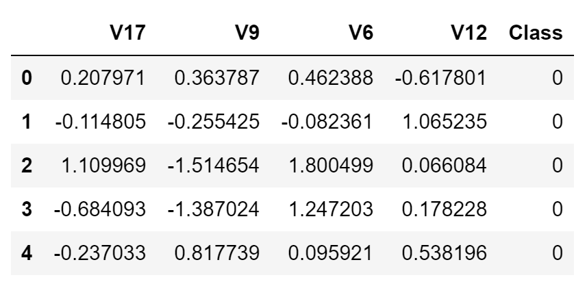
In order to demonstrate how to perform Hyperparameters Optimization in Python, I decided to perform a complete Data Analysis of the Credit Card Fraud Detection Kaggle Dataset. Our objective in this article will be to correctly classify which credit card transactions should be labelled as fraudulent or genuine (binary classification). This Dataset has been anonymized before being distributed, therefore, the meaning of most of the features has not been disclosed.
In this case, I decided to use just a subset of the dataset, in order to speed up training times and make sure to achieve a perfect balance between the two different classes. Additionally, just a limited amount of features has been used to make the optimization tasks more challenging. The final dataset is shown in the figure below (Figure 2).
All the code used in this article (and more!) is available in my GitHub repository and Kaggle Profile.
Machine Learning
First of all, we need to divide our dataset into training and test sets.
Throughout this article, we will use a Random Forest Classifier as our model to optimize.
Random Forest models are formed by a large number of uncorrelated decision trees, which joint together constitute an ensemble. In Random Forest, each decision tree makes its own prediction and the overall model output is selected to be the prediction which appeared most frequently.
We can now start by calculating our base model accuracy.
[[110   6]
 [  6 118]]
              precision    recall  f1-score   support

           0       0.95      0.95      0.95       116
           1       0.95      0.95      0.95       124

    accuracy                           0.95       240
   macro avg       0.95      0.95      0.95       240
weighted avg       0.95      0.95      0.95       240
Using the Random Forest Classifier with the default scikit-learn parameters lead to 95% overall accuracy. Let’s see now if applying some optimization techniques we can achieve better accuracy.
Manual Search
When using Manual Search, we choose some model hyperparameters based on our judgment/experience. We then train the model, evaluate its accuracy and start the process again. This loop is repeated until a satisfactory accuracy is scored.
The main parameters used by a Random Forest Classifier are:
- criterion = the function used to evaluate the quality of a split.
- max_depth = maximum number of levels allowed in each tree.
- max_features = maximum number of features considered when splitting a node.
- min_samples_leaf = minimum number of samples which can be stored in a tree leaf.
- min_samples_split = minimum number of samples necessary in a node to cause node splitting.
- n_estimators = number of trees in the ensemble.
More information about Random Forest parameters can be found on the scikit-learn Documentation.
As an example of Manual Search, I tried to specify the number of estimators in our model. Unfortunately, this didn’t lead to any improvement in accuracy.
[[110   6]
 [  6 118]]
              precision    recall  f1-score   support

           0       0.95      0.95      0.95       116
           1       0.95      0.95      0.95       124

    accuracy                           0.95       240
   macro avg       0.95      0.95      0.95       240
weighted avg       0.95      0.95      0.95       240
Random Search
In Random Search, we create a grid of hyperparameters and train/test our model on just some random combination of these hyperparameters. In this example, I additionally decided to perform Cross-Validation on the training set.
When performing Machine Learning tasks, we generally divide our dataset in training and test sets. This is done so that to test our model after having trained it (in this way we can check it’s performances when working with unseen data). When using Cross-Validation, we divide our training set into N other partitions to make sure our model is not overfitting our data.
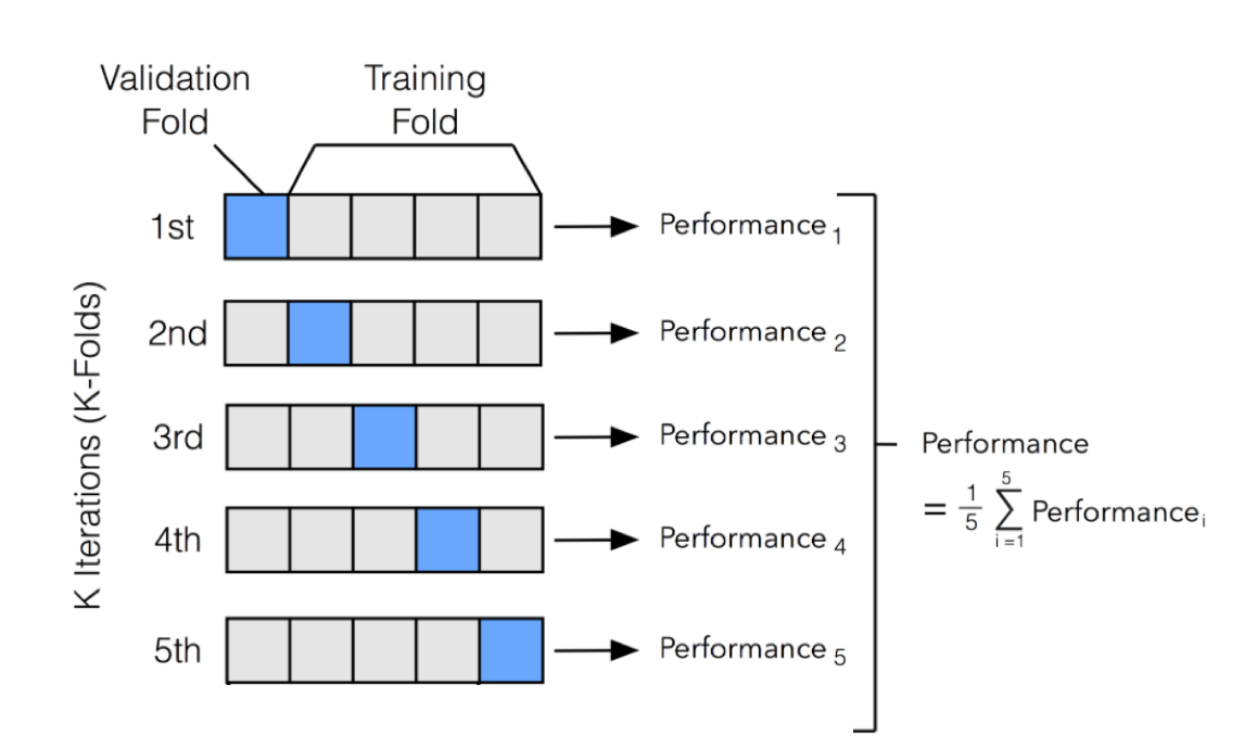
One of the most common used Cross-Validation methods is K-Fold Validation. In K-Fold, we divide our training set into N partitions and then iteratively train our model using N-1 partitions and test it with the left-over partition (at each iteration we change the left-over partition). Once having trained N times the model we then average the training results obtained in each iteration to obtain our overall training performance results (Figure 3).
Using Cross-Validation when implementing Hyperparameters optimization can be really important. In this way, we might avoid using some Hyperparameters which works really good on the training data but not so good with the test data.
We can now start implementing Random Search by first defying a grid of hyperparameters which will be randomly sampled when calling RandomizedSearchCV(). For this example, I decided to divide our training set into 4 Folds (cv = 4) and select 80 as the number of combinations to sample (n_iter = 80). Using the scikit-learn best_estimator_ attribute, we can then retrieve the set of hyperparameters which performed best during training to test our model.
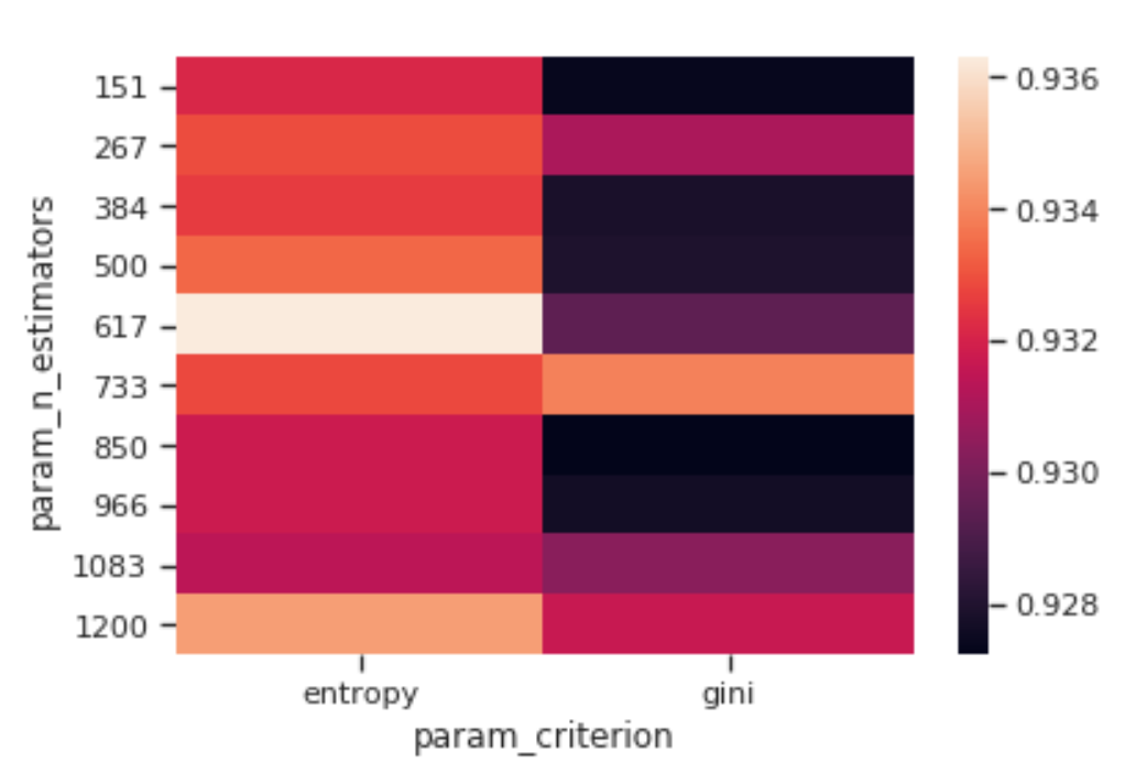
Once trained our model, we can then visualize how changing some of its Hyperparameters can affect the overall model accuracy (Figure 4). In this case, I decided to observe how changing the number of estimators and the criterion can affect our Random Forest accuracy.
We can then take this a step further by making our visualization more interactive. In the chart below, we can examine (using the slider) how varying the number of estimators in our model can affect the overall accuracy of our model considered the selected min_split and min_leaf parameters.
Feel free to play with the graph below by changing the n_estimators parameters, zooming in and out of the graph, changing it’s orientation and hovering over the single data points to get additional information about them!
If you are interested in finding out more about how to create these animations using Plotly, my code is available here. Additionally, this has also been covered in an article written by Xoel López Barata.
We can now evaluate how our model performed using Random Search. In this case, using Random Search leads to a consistent increase in accuracy compared to our base model.
[[115   1]
 [  6 118]]
              precision    recall  f1-score   support

           0       0.95      0.99      0.97       116
           1       0.99      0.95      0.97       124

    accuracy                           0.97       240
   macro avg       0.97      0.97      0.97       240
weighted avg       0.97      0.97      0.97       240
Grid Seach
In Grid Search, we set up a grid of hyperparameters and train/test our model on each of the possible combinations.
In order to choose the parameters to use in Grid Search, we can now look at which parameters worked best with Random Search and form a grid based on them to see if we can find a better combination.
Grid Search can be implemented in Python using scikit-learn GridSearchCV() function. Also on this occasion, I decided to divide our training set into 4 Folds (cv = 4).
When using Grid Search, all the possible combinations of the parameters in the grid are tried. In this case, 128000 combinations (2 × 10 × 4 × 4 × 4 × 10) will be used during training. Instead, in the Grid Search example before, just 80 combinations have been used.
[[115   1]
 [  7 117]]
              precision    recall  f1-score   support

           0       0.94      0.99      0.97       116
           1       0.99      0.94      0.97       124

    accuracy                           0.97       240
   macro avg       0.97      0.97      0.97       240
weighted avg       0.97      0.97      0.97       240
Grid Search is slower compared to Random Search but it can be overall more effective because it can go through the whole search space. Instead, Random Search can be faster fast but might miss some important points in the search space.
Automated Hyperparameter Tuning
When using Automated Hyperparameter Tuning, the model hyperparameters to use are identified using techniques such as: Bayesian Optimization, Gradient Descent and Evolutionary Algorithms.
Bayesian Optimization
Bayesian Optimization can be performed in Python using the Hyperopt library. Bayesian optimization uses probability to find the minimum of a function. The final aim is to find the input value to a function which can give us the lowest possible output value.
Bayesian optimization has been proved to be more efficient than random, grid or manual search. Bayesian Optimization can, therefore, lead to better performance in the testing phase and reduced optimization time.
In Hyperopt, Bayesian Optimization can be implemented giving 3 three main parameters to the function fmin().
- Objective Function = defines the loss function to minimize.
- Domain Space = defines the range of input values to test (in Bayesian Optimization this space creates a probability distribution for each of the used Hyperparameters).
- Optimization Algorithm = defines the search algorithm to use to select the best input values to use in each new iteration.
Additionally, can also be defined in fmin() the maximum number of evaluations to perform.
Bayesian Optimization can reduce the number of search iterations by choosing the input values bearing in mind the past outcomes. In this way, we can concentrate our search from the beginning on values which are closer to our desired output.
We can now run our Bayesian Optimizer using the fmin() function. A Trials() object is first created to make possible to visualize later what was going on while the fmin() function was running (eg. how the loss function was changing and how to used Hyperparameters were changing).
100%|██████████| 80/80 [03:07<00:00,  2.02s/it, best loss: -0.9339285714285713]{'criterion': 1,
 'max_depth': 120.0,
 'max_features': 2,
 'min_samples_leaf': 0.0006380325074247448,
 'min_samples_split': 0.06603114636418073,
 'n_estimators': 1}
We can now retrieve the set of best parameters identified and test our model using the best dictionary created during training. Some of the parameters have been stored in the best dictionary numerically using indices, therefore, we need first to convert them back as strings before input them in our Random Forest.
The classification report using Bayesian Optimization is shown below.
[[114   2]
 [ 11 113]]
              precision    recall  f1-score   support

           0       0.91      0.98      0.95       116
           1       0.98      0.91      0.95       124

    accuracy                           0.95       240
   macro avg       0.95      0.95      0.95       240
weighted avg       0.95      0.95      0.95       240
Genetic Algorithms
Genetic Algorithms tries to apply natural selection mechanisms to Machine Learning contexts. They are inspired by the Darwinian process of Natural Selection and they are therefore also usually called as Evolutionary Algorithms.
Let’s imagine we create a population of N Machine Learning models with some predefined Hyperparameters. We can then calculate the accuracy of each model and decide to keep just half of the models (the ones that perform best). We can now generate some offsprings having similar Hyperparameters to the ones of the best models so that to get again a population of N models. At this point, we can again calculate the accuracy of each model and repeat the cycle for a defined number of generations. In this way, just the best models will survive at the end of the process.
In order to implement Genetic Algorithms in Python, we can use the TPOT Auto Machine Learning library. TPOT is built on the scikit-learn library and it can be used for either regression or classification tasks.
The training report and the best parameters identified using Genetic Algorithms are shown in the following snippet.
Generation 1 - Current best internal CV score: 0.9392857142857143
Generation 2 - Current best internal CV score: 0.9392857142857143
Generation 3 - Current best internal CV score: 0.9392857142857143
Generation 4 - Current best internal CV score: 0.9392857142857143
Generation 5 - Current best internal CV score: 0.9392857142857143

Best pipeline: RandomForestClassifier(CombineDFs(input_matrix, input_matrix), criterion=entropy, max_depth=406, max_features=log2, min_samples_leaf=4, min_samples_split=5, n_estimators=617)
The overall accuracy of our Random Forest Genetic Algorithm optimized model is shown below.
0.9708333333333333
Artificial Neural Networks (ANNs) Tuning
Using KerasClassifier wrapper, it is possible to apply Grid Search and Random Search for Deep Learning models in the same way it was done when using scikit-learn Machine Learning models. In the following example, we will try to optimize some of our ANN parameters such as: how many neurons to use in each layer and which activation function and optimizer to use. More examples of Deep Learning Hyperparameters optimization are available here.
Max Accuracy Registred: 0.932 using {'activation': 'relu', 'neurons': 35, 'optimizer': 'Adam'}
The overall accuracy scored using our Artificial Neural Network (ANN) can be observed below.
[[115   1]
 [  8 116]]
              precision    recall  f1-score   support

           0       0.93      0.99      0.96       116
           1       0.99      0.94      0.96       124

    accuracy                           0.96       240
   macro avg       0.96      0.96      0.96       240
weighted avg       0.96      0.96      0.96       240
Evaluation
We can now compare how all the different optimization techniques performed on this given exercise. Overall, Random Search and Evolutionary Algorithms performed best.
Base Accuracy vs Manual Search 0.0000%.
Base Accuracy vs Random Search 2.1930%.
Base Accuracy vs Grid Search 1.7544%.
Base Accuracy vs Bayesian Optimization Accuracy -0.4386%.
Base Accuracy vs Evolutionary Algorithms 2.1930%.
Base Accuracy vs Optimized ANN 1.3158%.
The results obtained, are highly dependent on the chosen grid space and dataset used. Therefore, in different situations, different optimization techniques will perform better than others.
I hope you enjoyed this article, thank you for reading!
Contacts
If you want to keep updated with my latest articles and projects follow me on Medium and subscribe to my mailing list. These are some of my contacts details:
Bibliography
[1] Hyperparameter optimization: Explanation of automatized algorithms, Dawid Kopczyk. Accessed at: https://dkopczyk.quantee.co.uk/hyperparameter-optimization/
[2] Model Selection, ethen8181. Accessed at: http://ethen8181.github.io/machine-learning/model_selection/model_selection.html
Bio: Pier Paolo Ippolito is a final year MSc Artificial Intelligence student at The University of Southampton. He is an AI Enthusiast, Data Scientist and RPA Developer.
Original. Reposted with permission.
Related:
- Automated Machine Learning Project Implementation Complexities
- Automated Machine Learning: How do teams work together on an AutoML project?
- How to Automate Hyperparameter Optimization