Gradient Descent: The Mountain Trekker’s Guide to Optimization with Mathematics
Gradient descent is an optimization technique used to minimise errors in machine learning models. By iteratively adjusting parameters in the steepest direction of decrease, it seeks the lowest error value.
The Mountain Trekker Analogy:
Imagine you're a mountain trekker, standing somewhere on the slopes of a vast mountain range. Your goal is to reach the lowest point in the valley, but there's a catch: you're blindfolded. Without the ability to see the entire landscape, how would you find your way to the bottom?
Instinctively, you might feel the ground around you with your feet, sensing which way is downhill. You'd then take a step in that direction, the steepest descent. Repeating this process, you'd gradually move closer to the valley's lowest point.
Translating the Analogy to Gradient Descent
In the realm of machine learning, this trekker's journey mirrors the gradient descent algorithm. Here's how:
1) The Landscape: The mountainous terrain represents our cost (or loss) function,
J(θ). This function measures the error or discrepancy between our model's predictions and the actual data. Mathematically, it could be represented as:
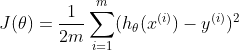
where
m is the number of data points,hθ(x) is our model's prediction, and
y is the actual value.
2) The Trekker's Position: Your current position on the mountain corresponds to the current values of the model's parameters,θ. As you move, these values change, altering the model's predictions.
3) Feeling the Ground: Just as you sense the steepest descent with your feet, in gradient descent, we compute the gradient,
∇J(θ). This gradient tells us the direction of the steepest increase in our cost function. To minimise the cost, we move in the opposite direction. The gradient is given by:
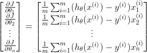
Where:
m is the number of training examples.
 is the prediction for the ith
training example.
 is the jth feature value for the ith training example.
 is the actual output for the ith
training example.
4) Steps: The size of the steps you take is analogous to the learning rate in gradient descent, denoted by ?. A large step might help you descend faster but risks overshooting the valley's bottom. A smaller step is more cautious but might take longer to reach the minimum. The update rule is:

5) Reaching the Bottom: The iterative process continues until you reach a point where you feel no significant descent in any direction. In gradient descent, this is when the change in the cost function becomes negligible, indicating that the algorithm has (hopefully) found the minimum.
In Conclusion
Gradient descent is a methodical and iterative process, much like our blindfolded trekker trying to find the valley's lowest point. By combining intuition with mathematical rigor, we can better understand how machine learning models learn, adjust their parameters, and improve their predictions.
Batch Gradient Descent
Batch Gradient Descent computes the gradient using the entire dataset. This method provides a stable convergence and consistent error gradient but can be computationally expensive and slow for large datasets.
Stochastic Gradient Descent (SGD)
SGD estimates the gradient using a single, randomly chosen data point. While it can be faster and is capable of escaping local minima, it has a more erratic convergence pattern due to its inherent randomness, potentially leading to oscillations in the cost function.
Mini-Batch Gradient Descent
Mini-Batch Gradient Descent strikes a balance between the two aforementioned methods. It computes the gradient using a subset (or "mini-batch") of the dataset. This method accelerates convergence by benefiting from the computational advantages of matrix operations and offers a compromise between the stability of Batch Gradient Descent and the speed of SGD.
Challenges and Solutions
Local Minima
Gradient descent can sometimes converge to a local minimum, which is not the optimal solution for the entire function. This is particularly problematic in complex landscapes with multiple valleys. To overcome this, incorporating momentum helps the algorithm navigate through valleys without getting stuck. Additionally, advanced optimization algorithms like Adam combine the benefits of momentum and adaptive learning rates to ensure more robust convergence to global minima.
Vanishing & Exploding Gradients
In deep neural networks, as gradients are back-propagated, they can diminish to near zero (vanish) or grow exponentially (explode). Vanishing gradients slow down training, making it hard for the network to learn, while exploding gradients can cause the model to diverge. To mitigate these issues, gradient clipping sets a threshold value to prevent gradients from becoming too large. On the other hand, normalized initialization techniques, like He or Xavier initialization, ensure that the weights are set to optimal values at the start, reducing the risk of these challenges.
Example Code for Gradient Descent Algorithm
import numpy as np

def gradient_descent(X, y, learning_rate=0.01, num_iterations=1000):
    m, n = X.shape
    theta = np.zeros(n)  # Initialize weights/parameters
    cost_history = []  # To store values of the cost function over iterations

    for _ in range(num_iterations):
        predictions = X.dot(theta)
        errors = predictions - y
        gradient = (1/m) * X.T.dot(errors)
        theta -= learning_rate * gradient

        # Compute and store the cost for current iteration
        cost = (1/(2*m)) * np.sum(errors**2)
        cost_history.append(cost)

    return theta, cost_history

# Example usage:
# Assuming X is your feature matrix with m samples and n features
# and y is your target vector with m samples.
# Note: You should add a bias term (column of ones) to X if you want a bias term in your model.

# Sample data
X = np.array([[1, 1], [1, 2], [1, 3], [1, 4], [1, 5]])
y = np.array([2, 4, 5, 4, 5])

theta, cost_history = gradient_descent(X, y)

print("Optimal parameters:", theta)
print("Cost history:", cost_history)
This code provides a basic gradient descent algorithm for linear regression. The function gradient_descent takes in the feature matrix X, target vector y, a learning rate, and the number of iterations. It returns the optimized parameters (theta) and the history of the cost function over the iterations.
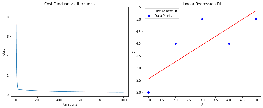
The left subplot shows the cost function decreasing over iterations.
The right subplot shows the data points and the line of best fit obtained from gradient descent.
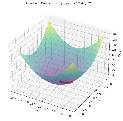
a 3D plot of the function  and overlay the path taken by gradient descent in red. The gradient descent starts from a random point and moves towards the minimum of the function.
Applications
Stock Price Prediction
Financial analysts use gradient descent in conjunction with algorithms like linear regression to predict future stock prices based on historical data. By minimising the error between the predicted and actual stock prices, they can refine their models to make more accurate predictions.
Image Recognition
Deep learning models, especially Convolutional Neural Networks (CNNs), employ gradient descent to optimise weights while training on vast datasets of images. For instance, platforms like Facebook use such models to automatically tag individuals in photos by recognizing facial features. The optimization of these models ensures accurate and efficient facial recognition.
Sentiment Analysis
Companies use gradient descent to train models that analyse customer feedback, reviews, or social media mentions to determine public sentiment about their products or services. By minimising the difference between predicted and actual sentiments, these models can accurately classify feedback as positive, negative, or neutral, helping businesses gauge customer satisfaction and tailor their strategies accordingly.
Arun is a seasoned Senior Data Scientist with over 8 years of experience in harnessing the power of data to drive impactful business solutions. He excels in leveraging advanced analytics, predictive modelling, and machine learning to transform complex data into actionable insights and strategic narratives. Holding a PGP in Machine Learning and Artificial Intelligence from a renowned institution, Arun's expertise spans a broad spectrum of technical and strategic domains, making him a valuable asset in any data-driven endeavour.