The Explainable Boosting Machine

By Dr. Robert Kübler, Data Scientist at Publicis Media

The Interpretability-Accuracy Trade-Off

 
In the machine learning community, I often hear and read about the notions of interpretability and accuracy, and how there is a trade-off between them. Usually, it is somewhat depicted like this:

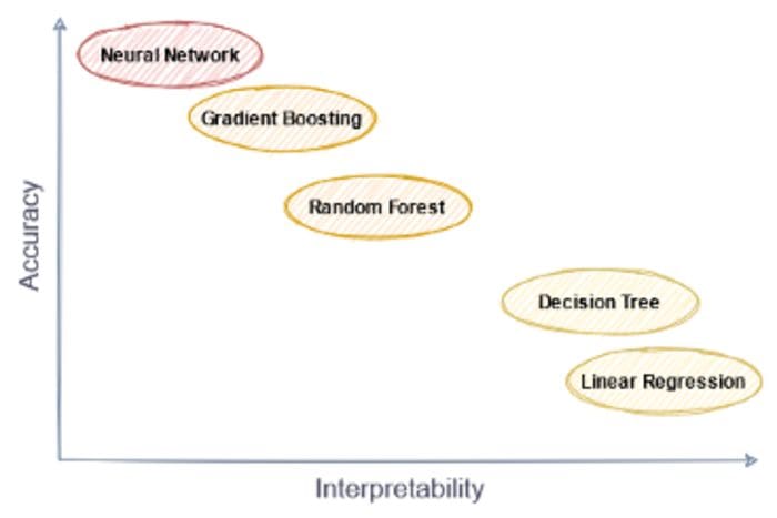
Image by the author.

You can read it as follows: Linear regression and decision trees are quite simple models which are not that accurate in general. Neural networks are black-box models, i.e. they are hard to interpret but perform quite decently in general. Ensemble models like random forests and gradient boosting are also good, but hard to interpret.

Interpretability

 
But what is interpretability anyway? There is no clear mathematical definition for that. Some authors such as in [1] and [2] define interpretability as the property that a human can understand and/or predict a model’s output. It is a bit wishy-washy but we can still kind of categorize machine learning models according to this.

Why is linear regression y=ax+b+ɛ interpretable? Because you can say something like “increasing x by one increases the outcome by a”. The model does not give you an unexpected output. The larger x, the larger y. The smaller x the smaller y. There are no inputs x that would let y wiggle around in a weird way.

Why are neural networks not interpretable? Well, try to guess the output of a 128 layer deep neural network without actually implementing it and without using pen and paper. Sure, the output is what it is according to some big formula, but even if I told you that for x=1 the output is y=10 and for x=3 the output is y=12, you would not be able to guess the output of x=2. Might be 11, might be -420.

Accuracy

 
That is what you are comfortable with — raw numbers. For regression, mean squared error, mean absolute error, mean absolute percentage error, you name it. For classification, F1, precision, recall, and, of course, the good old King Accuracy himself.

Let’s get back to the picture. While I agree with it as is, I want to stress the following:

There is no inherent trade-off between interpretability and accuracy. There are models that are both interpretable and accurate.

So, don’t let this picture fool you. Explainable Boosting Machines will help us break out from the middle, downward-sloping line and reach the holy grail that is the top right corner of our diagram.

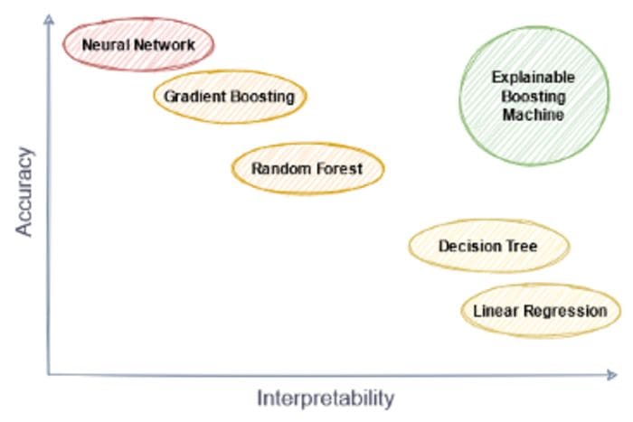
Image by the author.

(Of course, you can also create models that are both inaccurate and hard to interpret as well. This is an exercise you can do on your own.)

After reading this article you will be able to

• understand why interpretability matters,
• explain the drawbacks of black-box explanations such as LIME and Shapley values, and
• understand and use the Explainable Boosting Machine learner

Importance of Interpretation

 
Being able to interpret models has several benefits. It can help you improve the model, sometimes it is even required from the business, plain and simple.

Model improvement

Photo by alevision.co on Unsplash

Let’s imagine that you want to build a model to predict the price of a house. Creative, right? One of the input features is, among others, the number of rooms. Other features include the size, year build, and some measure of the quality of the neighborhood. After normalizing the features, you decided to use linear regression. The r² on the test set is nice and you deploy the model. At a later point, new house data comes in and you notice that your model is quite off. What went wrong?

Since linear regression is highly interpretable, you see the answer directly: the coefficient of the feature “number of rooms” is negative, although as a human you would expect it to be positive. The more rooms, the better, right? But the model learned the opposite for some reason.

There could be many reasons for this. Maybe your train and test set was biased in the way that if a house had more rooms, it tended to be older. And if a house is older, it tends to be cheaper.

This is something that you were only able to spot because you could take a look at how the model works inside. And not only you can spot it, but also fix it: you could set the coefficient of “number of rooms” to zero, or you could also retrain the model and enforce the coefficient of “number of rooms” to be positive. This is something you can do with scikit-learns LinearRegression by setting the keyword positive=True .

Note, however, that this sets all coefficients to be positive. You have to write your own linear regression, if you want complete control over the coefficients. You can check out this article to get started.

Business or regulatory requirement

Photo by Tingey Injury Law Firm on Unsplash

Often, stakeholders want to have at least some intuition on why things work, and you have to be able to explain it to them. While even the most non-technical people can agree on “I add together a bunch of numbers” (linear regression) or “I walk down a path and go left or right depending on some simple condition” (decision trees), it’s much more difficult for neural networks or ensemble methods. What the farmer doesn’t know he doesn’t eat. And it’s understandable because often these stakeholders have to report to other people, which in turn also want an explanation on how things roughly work. Good luck explaining gradient boosting to your boss in such a way that he or she can pass on the knowledge to a higher instance without doing any major mistake.

Besides that, interpretability may even be required by law. If you work for a bank and create a model that decides whether a person gets a loan or not, chances are that you are legally required to create an interpretable model, which might be logistic regression.

Before we cover the explainable boosting machine, let us take a look at some methods to interpret black-box models.

Interpretations of Black-Box Models

Photo by Laura Chouette on Unsplash

There are several ways that try to explain the workings of black-box models. The advantages of all of these methods are that you can take your already trained model and train some explainer on top of it. These explainers make the model easier to understand.

Famous examples of such explainers are Local interpretable model-agnostic explanations (LIME) [3] and Shapley values [4]. Let us quickly shed some light on the shortcomings of both of these methods.

Shortcomings of LIME

 
In LIME, you try to explain a single prediction of your model at a time. Given a sample x, why is the label y? The assumption is that you can approximate your complicated black-box model with an interpretable model in a close region around x. This model is called a surrogate model, and often linear/logistic regressions or decision trees are chosen for this. However, if the approximation is bad, which you might not notice, the explanations become misleading.

It’s still a sweet library that you should be aware of.

Shapley values

 
With Shapley values, each prediction can be broken down into individual contributions for every feature. As an example, if your model outputs a 50, with Shapley values you can say that feature 1 contributed 10, feature 2 contributed 60, feature 3 contributed -20. The sum of these 3 Shapley values is 10+60–20=50, the output of your model. This is great, but sadly, these values are extremely hard to calculate.

For a general black-box model, the run-time for computing them is exponential in the number of features. If you have a few features, like 10, this might still be okay. But, depending on your hardware, for 20 it might be impossible already. To be fair, if your black-box model consists of trees, there are faster approximations to compute Shapley values, but it can still be slow.

Still, there is the great shap library for Python that can compute Shapley values, and that you should definitely check out!

Don’t get me wrong. Black-box explanations are much better than no explanation at all, so use them, if you have to use a black-box model for some reason. But of course, it would be better if your model is performing well and is interpretable at the same time. It is finally time to move on to a representative of such methods.

Explainable Boosting Machine

 
The fundamental idea of explainable boosting is nothing new at all. It started out with additive models, pioneered by Jerome H. Friedman and Werner Stuetzle in 1981 already. Models of this kind have the following form:

Image by the author.

where y is the prediction and x₁, …, xₖ are the input features.

An old friend

 
I claim that all of you have stumbled across such a model already. Let’s say it out loud:

Linear Regression!

Linear regression is nothing else but a special kind of additive model. Here, all functions fᵢ are just the identity, i.e. fᵢ(xᵢ)=xᵢ. Easy, right? But you also know that linear regression might not be the best option in terms of accuracy if its assumptions, especially the linearity assumption, are violated.

What we need are more general functions that can capture more complicated correlations between input and output variables. An interesting example of how to do design such functions was presented by some people at Microsoft [5]. Even better: they have built a comfortable package for Python and even R around this idea.

Note that in the following I will only describe the explainable boosting regressor. Classifying works as well and is not much more complicated.

Interpretation

 
You might say:

With these functions f, this looks more complicated than linear regression. How is this easier to interpret?

To illustrate this, assume that we have trained an additive model that looks like this:

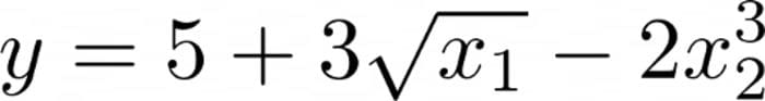
Image by the author.

You can plug in (16, 2) into the model and receive 5+12–16=1 as an output. And this is the output of 1 broken down already — there is a baseline of 5, then feature 1 provides an additional 12, and feature 3 provides an additional -16.

The fact that all functions, even if they are complicated, are just composed by simple addition makes this model so easy to interpret.

Let us now see how this model works.

The idea

 
The authors use small trees in a way that resembles gradient boosting. Please, refer to this great video if you don’t know how gradient boosting works.

Now, instead of training each of the small trees on all features, the authors of the explainable boosting regressor propose training each small tree with one feature at a time. This creates a model that looks like this:

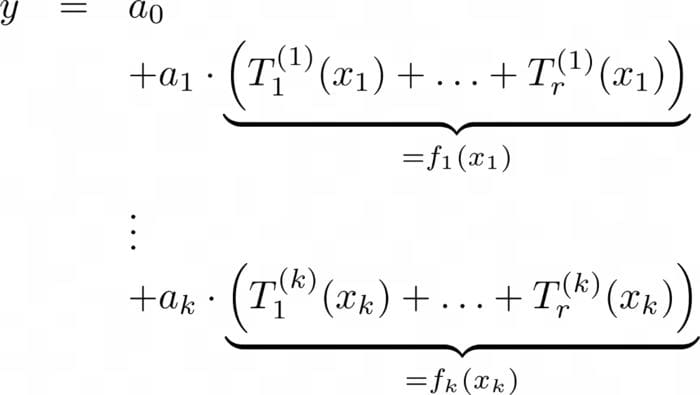
Image by the author.

You can see the following here:

• Each T is a tree with a small depth.
• For each of the k features, r trees are trained. Therefore, you can see k*r different trees in the equation.
• For each feature, the sum of all of its trees is the aforementioned f.

This means that the functions f are composed of sums of small trees. As trees are quite versatile, many complicated functions can be modeled quite accurately.

Make also sure to check out this video for an alternative explanation:

Alright, we have seen how it works and that you can interpret the outputs of explainable boosting machines easily. But are these models any good? Their paper [5] says the following:

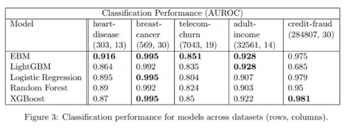
Image is taken from [5]. EBM = Explainable Boosting Machine.

Looks good to me! Of course, I also tested this algorithm, and it has been effective on my datasets as well. Speaking of testing, let us see how to actually use explainable boosting in Python.

Using explainable boosting in Python

 
Microsoft’s interpret package makes using explainable boosting a breeze, as is it uses the scikit-learn API. Here is a small example:

from interpret.glassbox import ExplainableBoostingRegressor
from sklearn.datasets import load_bostonX, y = load_boston(return_X_y=True)
ebm = ExplainableBoostingRegressor()
ebm.fit(X, y)

Nothing surprising here. But the interpret package has much more to offer. I especially like the visualization tools.

from interpret import showshow(ebm.explain_global())

Among other things, the show method lets you even inspect the functions f. Here is the one for feature 4 (NOX; nitric oxides concentration) of the Boston housing dataset.

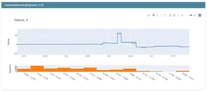
Image by the author.

Here, you can see that up to about 0.58, there is no influence of NOX on the house price. Starting from 0.58, the influence gets slightly positive, and NOX values around 0.62 have the highest positive influence on the house price. Then it dips again until the influence becomes negative for NOX values larger than 0.66.

Conclusion

 
In this article, we have seen that interpretability is a desirable property. If our models are not interpretable by default, we can still help ourselves with methods such as LIME and Shapley values. This is better than doing nothing, but also these methods have their shortcomings.

We then introduced the explainable boosting machine, which has an accuracy that is comparable to gradient boosting algorithms such as XGBoost and LightGBM, but is interpretable as well. This shows that accuracy and interpretability as not mutually exclusive.

Using explainable boosting in production is not difficult, thanks to the interpret package.

Slight room for improvement

 
It’s a great library that has only one major drawback at the moment: It only supports trees as base learners. This might be enough most of the time, but if you require monotone functions, for example, you are alone at the moment. However, I think it should be easy to implement this: The developers only have to add only two features:

1. Support for general base learners. Then we can use isotonic regression to create monotone functions.
2. Support for different base learners for different features. Because for some features you want your function f to be monotonically increasing, for others decreasing, and for some, you do not care.

You can view the discussion here.

References

 
[1] Miller, T. (2019). Explanation in artificial intelligence: Insights from the social sciences. Artificial intelligence, 267, 1–38.

[2] Kim, B., Koyejo, O., & Khanna, R. (2016, December). Examples are not enough, learn to criticize! Criticism for Interpretability. In NIPS (pp. 2280–2288).

[3] Ribeiro, M. T., Singh, S., & Guestrin, C. (2016, August). “Why should i trust you?” Explaining the predictions of any classifier. In Proceedings of the 22nd ACM SIGKDD international conference on knowledge discovery and data mining (pp. 1135–1144).

[4] Lundberg, S., & Lee, S. I. (2017). A unified approach to interpreting model predictions. arXiv preprint arXiv:1705.07874.

[5] Nori, H., Jenkins, S., Koch, P., & Caruana, R. (2019). Interpretml: A unified framework for machine learning interpretability. arXiv preprint arXiv:1909.09223.

Thanks to Patrick Bormann for his useful remarks!

I hope that I could teach you something useful.

Thanks for reading!

If you have any questions, write me on LinkedIn!

Also, check out my other articles on graspable machine learning topics.

 
Bio: Dr. Robert Kübler is a Data Scientist at Publicis Media and Author at Towards Data Science.

Original. Reposted with permission.

Related:

• Gradient Boosted Decision Trees – A Conceptual Explanation
• Shapash: Making Machine Learning Models Understandable
• Interpretable Machine Learning: The Free eBook