Gradient Boosted Decision Trees – A Conceptual Explanation

Gradient boosted decision trees involves implementing several models and aggregating their results. These boosted models have become popular thanks to their performance in machine learning competitions on Kaggle. In this article, we’ll see what gradient boosted decision trees are all about.

By Derrick Mwiti, Data Scientist on April 30, 2021 in CatBoost, Decision Trees, Gradient Boosting, Machine Learning, Python, scikit-learn, XGBoost

comments

Gradient boosted decision trees have proven to outperform other models. It’s because boosting involves implementing several models and aggregating their results.

Gradient boosted models have recently become popular thanks to their performance in machine learning competitions on Kaggle.

In this article, we’ll see what gradient boosted decision trees are all about.

Gradient boosting

In gradient boosting, an ensemble of weak learners is used to improve the performance of a machine learning model. The weak learners are usually decision trees. Combined, their output results in better models.

In case of regression, the final result is generated from the average of all weak learners. With classification, the final result can be computed as the class with the majority of votes from weak learners.

In gradient boosting, weak learners work sequentially. Each model tries to improve on the error from the previous model. This is different from the bagging technique, where several models are fitted on subsets of the data in a parallel manner. These subsets are usually drawn randomly with replacement. A great example of bagging is in Random Forests®.

The boosting process looks like this:

Build an initial model with the data,
Run predictions on the whole data set,
Calculate the error using the predictions and the actual values,
Assign more weight to the incorrect predictions,
Create another model that attempts to fix errors from the last model,
Run predictions on the entire dataset with the new model,
Create several models with each model aiming at correcting the errors generated by the previous one,
Obtain the final model by weighting the mean of all the models.

Boosting algorithms in machine learning

Let’s take a look at boosting algorithms in machine learning.

AdaBoost

AdaBoost fits a sequence of weak learners to the data. It then assigns more weight to incorrect predictions, and less weight to correct ones. This way the algorithm focuses more on observations that are harder to predict. The final result is obtained from the majority vote in classification, or the average in regression.

You can implement this algorithm using Scikit-learn. The `n_estimators` argument can be passed to it to indicate the number of weak learners needed. You can control the contribution of each weak learner using the `learning_rate` argument.

The algorithm uses decision trees as the base estimators by default. The base estimators and the parameters of the decision trees can be tuned to improve the performance of the model. By default, decision trees in AdaBoost have a single split.

Classification using AdaBoost

You can use the `AdaBoostClassifier` from Scikit-learn to implement the AdaBoost model for classification problems. As you can see below, the parameters of the base estimator can be tuned to your preference. The classifier also accepts the number of estimators you want. This is the number of decision trees you need for the model.

from sklearn.tree import DecisionTreeClassifier
from sklearn.ensemble import AdaBoostClassifier
base_estimator=DecisionTreeClassifier(max_depth=1,criterion='gini', splitter='best', min_samples_split=2)
model = AdaBoostClassifier(base_estimator=base_estimator,n_estimators=100)
model.fit(X_train, y_train)

Regression using AdaBoost

Applying AdaBoost to regression problems is similar to the classification process, with just a few cosmetic changes. First, you have to import the `AdaBoostRegressor`. Then, for the base estimator, you can use the `DecisionTreeRegressor`. Just like the previous one, you can tune the parameters of the decision tree regressor.

from sklearn.tree import DecisionTreeRegressor
from sklearn.ensemble import AdaBoostRegressor
base_estimator = DecisionTreeRegressor(max_depth=1, splitter='best', min_samples_split=2)
model = AdaBoostRegressor(base_estimator=base_estimator,n_estimators=100)
model.fit(X_train, y_train)

Scikit-learn gradient boosting estimator

Gradient boosting is different from AdaBoost, because the loss function optimization is done via gradient descent. Like AdaBoost, it also uses decision trees as weak learners. It also sequentially fits the trees. When adding subsequent trees, loss is minimized using gradient descent.

In the Scikit-learn implementation, you can specify the number of trees. This is a parameter that should be looked at keenly, because specifying too many trees can lead to overfitting. On the other hand, specifying a very small number of trees can lead to underfitting.

The algorithm lets you specify the learning rate. This dictates how fast the model will learn. A low learning rate will often require more trees in the model. This means more training time.

Let’s now take a look at the implementation of gradient boosted trees in Scikit-learn.

Classification with the Scikit-learn gradient boosting estimator

This is implemented using the `GradientBoostingClassifier`. Some of the parameters expected by this algorithm include:

`loss` defining the loss function to be optimized
`learning_rate` that determines the contribution of each tree
`n_estimatorst` dictates the number of decision trees
`max_depth` is the maximum depth of each estimator

from sklearn.ensemble import GradientBoostingClassifier
gbc = GradientBoostingClassifier(loss='deviance', learning_rate=0.1, n_estimators=100, subsample=1.0, criterion='friedman_mse', min_samples_split=2, min_samples_leaf=1)
gbc.fit(X_train,y_train)

After fitting the classifier, you can obtain the importance of the features using the `feauture_importances_` attribute. This is usually referred to as the Gini importance.

gbc.feature_importances_

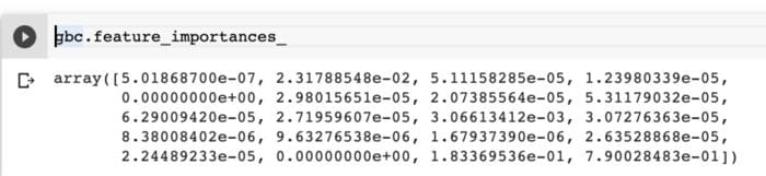
Gradient boosted decision tree feature import

The higher the value, the more important the feature is. The values in the obtained array will sum to 1.

Note: Impurity-based importances are not always accurate, especially when there are too many features. In that case, you should consider using permutation-based importances.

Regression with the Scikit-learn gradient boosting estimator

The Scikit-learn gradient boosting estimator can be implemented for regression using `GradientBoostingRegressor`. It takes parameters that are similar to the classification one:

loss,
number of estimators,
maximum depth of the trees,
learning rate…

…just to mention a few.

from sklearn.ensemble import GradientBoostingRegressor
params = {'n_estimators': 500,
          'max_depth': 4,
          'min_samples_split': 5,
          'learning_rate': 0.01,
          'loss': 'ls'}
gbc = GradientBoostingRegressor(**params)
gbc.fit(X_train,y_train)

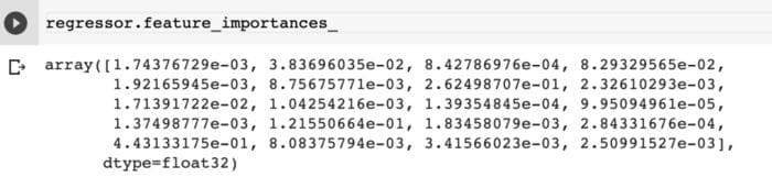
Like the classification model, you can also obtain the feature importances for the regression algorithm.

gbc.feature_importances_

XGBoost

XGBoost is a gradient boosting library supported for Java, Python, Java and C++, R, and Julia. It also uses an ensemble of weak decision trees.

It’s a linear model that does tree learning through parallel computations. The algorithm also ships with features for performing cross-validation, and showing the feature’s importance. The main features of this model are:

accepts sparse input for tree booster and linear booster,
supports custom evaluation and objective functions,
`Dmatrix`, its optimized data structure improves its performance.

Let’s take a look at how you can apply XGBoost in Python. The parameters accepted by the algorithm include:

`objective` to define the type of task, say regression or classification;
`colsample_bytree` the subsample ratio of columns when constructing each tree. Subsampling happens once in every iteration. This number is usually a value between 0 and 1;
`learning_rate` that determines how fast or slow the model will learn;
`max_depth` indicates the maximum depth for each tree. The more the trees, the greater model complexity, and the higher chances of overfitting;
`alpha` is the L1 regularization on weights;
`n_estimators` is the number of decision trees to fit.

Classification with XGBoost

After importing the algorithm, you define the parameters that you would like to use. Since this is a classification problem, the `binary: logistic` objective function is used. The next step is to use the `XGBClassifier` and unpack the defined parameters. You can tune these parameters until you obtain the ones that are optimal for your problem.

import xgboost as xgb
params = {"objective":"binary:logistic",'colsample_bytree': 0.3,'learning_rate': 0.1,
                'max_depth': 5, 'alpha': 10}
classification = xgb.XGBClassifier(**params)
classification.fit(X_train, y_train)

Regression with XGBoost

In regression, the `XGBRegressor` is used instead. The objective function, in this case, will be the `reg:squarederror`.

import xgboost as xgb
params = {"objective":"reg:squarederror",'colsample_bytree': 0.3,'learning_rate': 0.1,
                'max_depth': 5, 'alpha': 10}
regressor = xgb.XGBRegressor(**params)
regressor.fit(X_train, y_train)

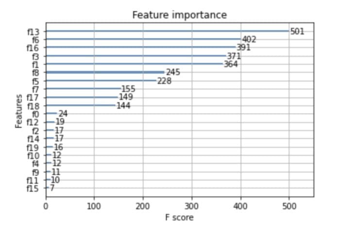
The XGBoost models also allow you to obtain the feature importances via the `feature_importances_` attribute.

regressor.feature_importances_

You can easily visualize them using Matplotlib. This is done using the `plot_importance` function from XGBoost.

import matplotlib.pyplot as plt
xgb.plot_importance(regressor)
plt.rcParams['figure.figsize'] = [5, 5]
plt.show()

The `save_model` function can be used for saving your model. You can then send this model to your model registry.

regressor.save_model("model.pkl")

Check Neptune docs about integration with XGBoost and with matplotlib.

LightGBM

LightGBM is different from other gradient boosting frameworks because it uses a leaf-wise tree growth algorithm. Leaf-wise tree growth algorithms are known to converge faster than depth-wise growth algorithms. However, they’re more prone to overfitting.

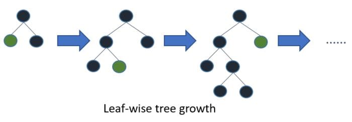Source

The algorithm is histogram-based, so it places continuous values into discrete bins. This leads to faster training and efficient memory utilization.

Other notable features from this algorithm include:

support for GPU training,
native support for categorical features,
ability to handle large-scale data,
handles missing values by default.

Let’s take a look at some of the main parameters of this algorithm:

`max_depth` the maximum depth of each tree;
`objective` which defaults to regression;
`learning_rate` the boosting learning rate;
`n_estimators` the number of decision trees to fit;
`device_type` whether you’re working on a CPU or GPU.

Classification with LightGBM

Training a binary classification model can be done by setting `binary` as the objective. If it’s a multi-classification problem, the `multiclass` objective is used.

The dataset is also converted to LightGBM’s `Dataset` format. Training the model is then done using the `train` function. You can also pass the validation datasets using the `valid_sets` parameter.

import lightgbm as lgb
lgb_train = lgb.Dataset(X_train, y_train)
lgb_eval = lgb.Dataset(X_test, y_test, reference=lgb_train)
params = {'boosting_type': 'gbdt',
              'objective': 'binary',
              'num_leaves': 40,
              'learning_rate': 0.1,
              'feature_fraction': 0.9
              }
gbm = lgb.train(params,
    lgb_train,
    num_boost_round=200,
    valid_sets=[lgb_train, lgb_eval],
    valid_names=['train','valid'],
   )

Regression with LightGBM

For regression with LightGBM, you just need to change the objective to `regression`. The boosting type is Gradient Boosting Decision Tree by default.

If you like, you can change this to the random forest algorithm, `dart` — Dropouts meet Multiple Additive Regression Trees, or `goss` — Gradient-based One-Side Sampling.

import lightgbm as lgb
lgb_train = lgb.Dataset(X_train, y_train)
lgb_eval = lgb.Dataset(X_test, y_test, reference=lgb_train)
params = {'boosting_type': 'gbdt',
              'objective': 'regression',
              'num_leaves': 40,
              'learning_rate': 0.1,
              'feature_fraction': 0.9
              }
gbm = lgb.train(params,
    lgb_train,
    num_boost_round=200,
    valid_sets=[lgb_train, lgb_eval],
    valid_names=['train','valid'],
   )

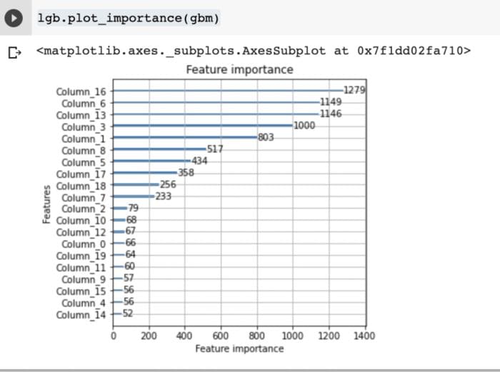
You can also use LightGBM to plot the model’s feature importance.

lgb.plot_importance(gbm)

LightGBM also has a built-in function for saving the model. That function is `save_model`.

gbm.save_model('mode.pkl')

CatBoost

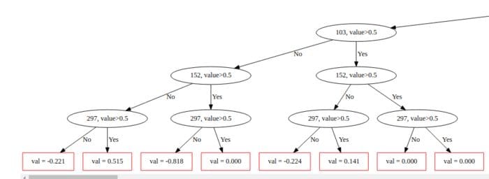
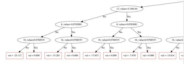
CatBoost is a depth-wise gradient boosting library developed by Yandex. The algorithm grows a balanced tree using oblivious decision trees.

It uses the same features to make the right and left split at each level of the tree.

For example in the image below, you can see that `297,value>0.5` is used through that level.

Other notable features of CatBoost include:

native support for categorical features,
supports training on multiple GPUs,
results in good performance with the default parameters,
fast prediction via CatBoost’s model applier,
handles missing values natively,
support for regression and classification problems.

Let’s now mention a couple of training parameters from CatBoost:

`loss_function` the loss to be used for classification or regression;
`eval_metric` the model’s evaluation metric;
`n_estimators` the maximum number of decision trees;
`learning_rate` determines how fast or slow the model will learn;
`depth` the maximum depth for each tree;
`ignored_features` determines the features that should be ignored during training;
`nan_mode` the method that will be used to deal with missing values;
`cat_features` an array of categorical columns;
`text_features` for declaring text-based columns.

Classification with CatBoost

For classification problems,`CatBoostClassifier` is used. Setting `plot=True` during the training process will visualize the model.

from catboost import CatBoostClassifier
model = CatBoostClassifier()
model.fit(X_train,y_train,verbose=False, plot=True)

Regression with CatBoost

In the case of regression, the `CatBoostRegressor` is used.

from catboost import CatBoostRegressor
model = CatBoostRegressor()
model.fit(X_train,y_train,verbose=False, plot=True)

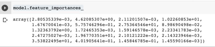
You can also use the `feature_importances_` to obtain the ranking of the features by their importance.

model.feature_importances_

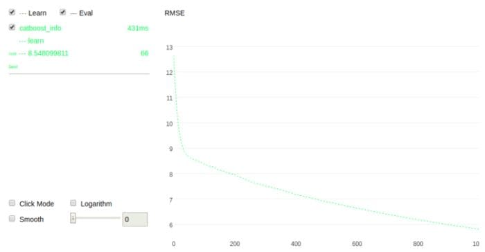
The algorithm also provides support for performing cross-validation. This is done using the `cv` function while passing the required parameters.

Passing `plot=”True”` will visualize the cross-validation process. The `cv` function expects the dataset to be in CatBoost’s `Pool` format.

from catboost import Pool, cv
params = {"iterations": 100,
          "depth": 2,
          "loss_function": "RMSE",
          "verbose": False}
cv_dataset = Pool(data=X_train,
                  label=y_train)
scores = cv(cv_dataset,
            params,
            fold_count=2, 
            plot=True)

You can also use CatBoost to perform a grid search. This is done using the `grid_search` function. After searching, CatBoost trains on the best parameters.

You should not have fitted the model before this process. Passing the `plot=True` parameter will visualize the grid search process.

grid = {'learning_rate': [0.03, 0.1],
        'depth': [4, 6, 10],
        'l2_leaf_reg': [1, 3, 5, 7, 9]}

grid_search_result = model.grid_search(grid, X=X_train, y=y_train, plot=True)

CatBoost also enables you to visualize a single tree in the model. This is done using the `plot_tree` function and passing the index of the tree you would like to visualize.

model.plot_tree(tree_idx=0)

Advantages of gradient boosting trees

There are several reasons as to why you would consider using gradient boosting tree algorithms:

generally more accurate compare to other modes,
train faster especially on larger datasets,
most of them provide support handling categorical features,
some of them handle missing values natively.

Disadvantages of gradient boosting trees

Let’s now address some of the challenges faced when using gradient boosted trees:

prone to overfitting: this can be solved by applying L1 and L2 regularization penalties. You can try a low learning rate as well;
models can be computationally expensive and take a long time to train, especially on CPUs;
hard to interpret the final models.

Final thoughts

In this article, we explored how to implement gradient boosting decision trees in your machine learning problems. We also walked through various boosting-based algorithms that you can start using right away.

Specifically, we’ve covered:

what is gradient boosting,
how gradient boosting works,
various types of gradient boosting algorithms,
how to use gradient boosting algorithms for regression and classification problems,
the advantages of gradient boosting trees,
disadvantages of gradient boosting trees,

…and so much more.

You’re all set to start boosting your machine learning models.

Resources

Bio: Derrick Mwiti is a data scientist who has a great passion for sharing knowledge. He is an avid contributor to the data science community via blogs such as Heartbeat, Towards Data Science, Datacamp, Neptune AI, KDnuggets just to mention a few. His content has been viewed over a million times on the internet. Derrick is also an author and online instructor. He also trains and works with various institutions to implement data science solutions as well as to upskill their staff. You might want to check his Complete Data Science & Machine Learning Bootcamp in Python course.

Original. Reposted with permission.

Related: