Decision Trees vs Random Forests, Explained
A simple, non-math heavy explanation of two popular tree-based machine learning models.
Introduction
Decision trees and random forests are two of the most popular predictive models for supervised learning. These models can be used for both classification and regression problems.
In this article, I will explain the difference between decision trees and random forests. By the end of the article, you should be familiar with the following concepts:
- How does the decision tree algorithm work?
- Components of a decision tree
- Pros and cons of the decision tree algorithm?
- What does bagging mean, and how does the random forest algorithm work?
- Which algorithm is better in terms of speed and performance
Decision Trees
Decision trees are highly interpretable machine learning models that allow us to stratify or segment data. They allow us to continuously split data based on specific parameters until a final decision is made.
How does the decision tree algorithm work?
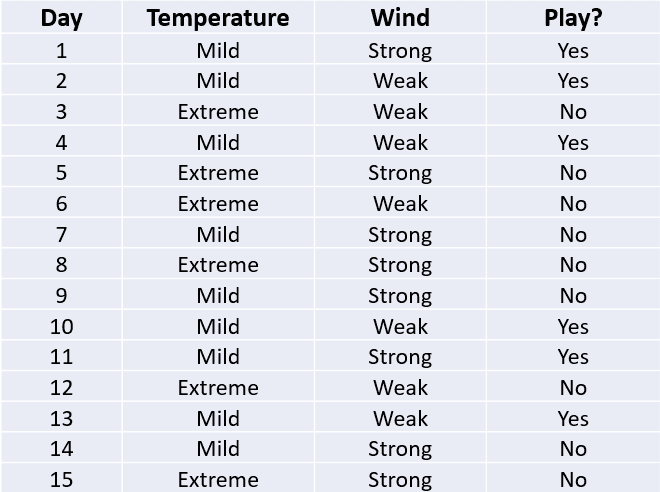
Take a look at the following table:
This dataset consists of only four variables?—?“Day”, ‘‘Temperature’’, ‘‘Wind’’, and ‘‘Play?’’. Depending on the temperature and wind on any given day, the outcome is binary - either to go out and play or stay home.
Let’s build a decision tree using this data:
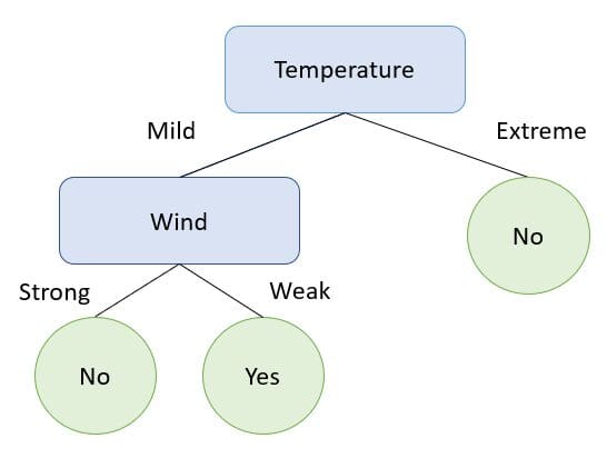
The example above is one that is simple, but encapsulates exactly how a decision tree splits on different data points until an outcome is obtained.
From the visualization above, notice that the decision tree splits on the variable “Temperature” first. It also stops splitting when the temperature is extreme, and says that we should not go out to play.
It is only if the temperature is mild that it starts to split on the second variable.
These observations lead to the following questions:
- How does a decision tree decide on the first variable to split on?
- How to decide when to stop splitting?
- What is the order used to construct a decision tree?
Entropy
Entropy is a metric that measures the impurity of a split in a decision tree. It determines how the decision tree chooses to partition data. Entropy values range from 0 to 1. A value of 0 indicates a pure split and a value of 1 indicates an impure split.
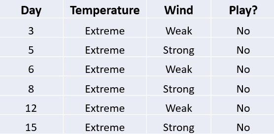
In the decision tree above, recall the tree had stopped splitting when the temperature was extreme:
This is because when the temperature is extreme, the outcome of “Play?” is always “No.” This means that we have a pure split with 100% of data points in a single class. The entropy value of this split is 0, and the decision tree will stop splitting on this node.
Decision trees will always select the feature with the lowest entropy to be the first node.
In this case, since the variable “Temperature” had a lower entropy value than “Wind”, this was the first split of the tree.
Watch this YouTube video to learn more about how entropy is calculated and how it is used in decision trees.
Information Gain
Information gain measures the reduction in entropy when building a decision tree.
Decision trees can be constructed in a number of different ways. The tree needs to find a feature to split on first, second, third, etc. Information gain is a metric that tells us the best possible tree that can be constructed to minimize entropy.
The best tree is one with the highest information gain.
If you’d like to learn more about how to calculate information gain and use it to build the best possible decision tree, you can watch this YouTube video.
Components of a decision tree:
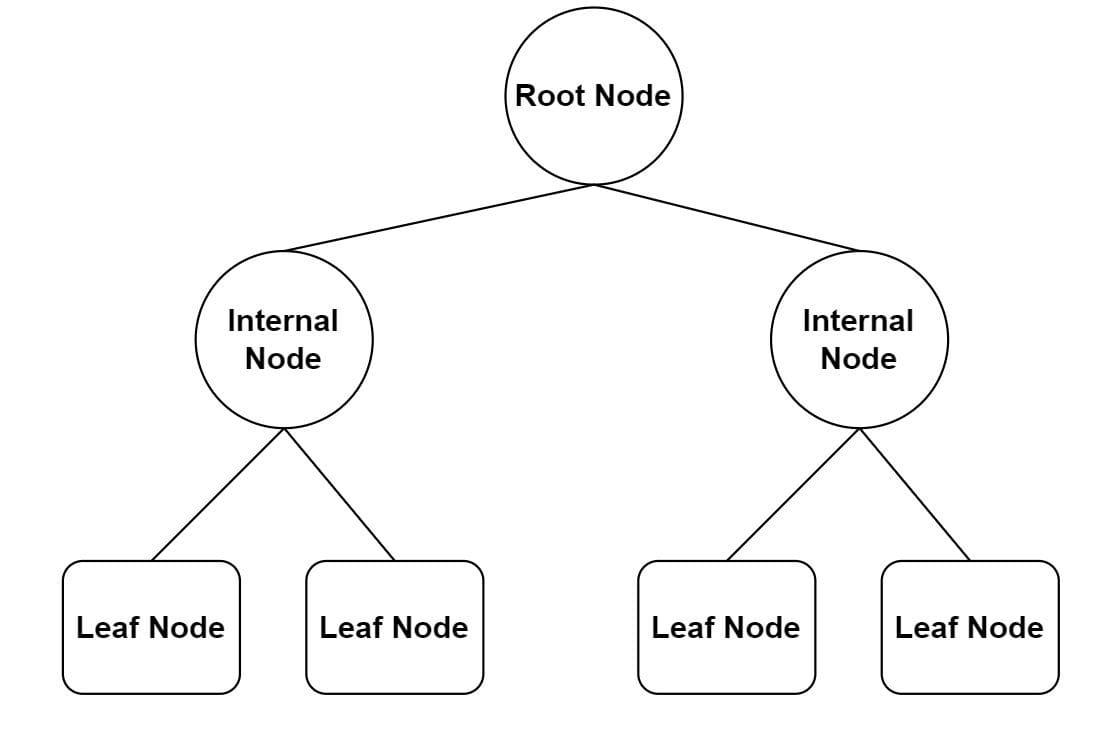
- Root node: A root node is at the top of the decision tree, and is the variable from which the dataset starts dividing. The root node is the feature that provides us with the best split of data.
- Internal nodes: These are the nodes that split the data after the root node.
- Leaf nodes: Finally, these are nodes at the bottom of the decision tree after which no further splits are possible.
- Branches: Branches connect one node to another and are used to represent the outcome of a test.
Pros and Cons of the Decision Tree Algorithm:
Now that you understand how decision trees work, let’s take a look at some advantages and disadvantages of the algorithm.
Pros
- Decision trees are simple and easy to interpret.
- They can be used for classification and regression problems.
- They can partition data that isn’t linearly separable.
Cons
- Decision trees are prone to overfitting.
- Even a small change in the training dataset can make a huge difference in the logic of decision trees.
Random Forests
One of the biggest drawbacks of the decision tree algorithm is that it is prone to overfitting. This means that the model is overly complex and has high variance. A model like this will have high training accuracy but will not generalize well to other datasets.
How does the random forest algorithm work?
The random forest algorithm solves the above challenge by combining the predictions made by multiple decision trees and returning a single output. This is done using an extension of a technique called bagging, or bootstrap aggregation.
Bagging is a procedure that is applied to reduce the variance of machine learning models. It works by averaging a set of observations to reduce variance.
Here is how bagging works:
Bootstrap
If we had more than one training dataset, we could train multiple decision trees on each dataset and average the results.
However, since we usually only have one training dataset in most real-world scenarios, a statistical technique called bootstrap is used to sample the dataset with replacement.
Then, multiple decision trees are created, and each tree is trained on a different data sample:
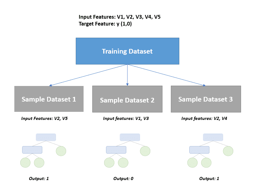
Notice that three bootstrap samples have been created from the training dataset above. The random forest algorithm goes a step further than bagging and randomly samples features so only a subset of variables are used to build each tree.
Each decision tree will render different predictions based on the data sample they were trained on.
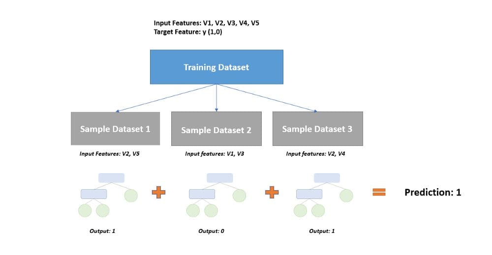
Aggregation
In this step, the prediction of each decision tree will be combined to come up with a single output.
In the case of a classification problem, a majority class prediction is made:
In regression problems, the predictions of all decision trees will be averaged to come up with a single value.
Why do we randomly sample variables in the random forest algorithm?
In the random forest algorithm, it is not only rows that are randomly sampled, but variables too.
This is because if we were to build multiple decision trees with the same features, every tree will be similar and highly correlated with each other, potentially yielding the same result. This will again lead to the issue of high variance.
Decision Trees vs. Random Forests - Which One Is Better and Why?
Random forests typically perform better than decision trees due to the following reasons:
- Random forests solve the problem of overfitting because they combine the output of multiple decision trees to come up with a final prediction.
- When you build a decision tree, a small change in data leads to a huge difference in the model’s prediction. With a random forest, this problem does not arise since the data is sampled many times before generating a prediction.
In terms of speed, however, the random forests are slower since more time is taken to construct multiple decision trees. Adding more trees to a random forest model will improve its accuracy to a certain extent, but also increases computation time.
Finally, decision trees are also easier to interpret than random forests since they are straightforward. It is easy to visualize a decision tree and understand how the algorithm reached its outcome. A random forest is harder to deconstruct since it is more complex and combines the output of multiple decision trees to make a prediction.
Natassha Selvaraj is a self-taught data scientist with a passion for writing. You can connect with her on LinkedIn.